21 SQL II

Learning Outcomes

Perform aggregations using GROUP BY
Introduce the ability to filter groups
Perform data cleaning and text manipulation in SQL
Join data across tables

In this lecture, we’ll continue our work from last time to introduce some advanced SQL syntax.

First, let’s load in the basic_examples.db database.

Code

# Load the SQL Alchemy Python library and DuckDB
import sqlalchemy
import duckdb

# Load %%sql cell magic
%load_ext sql

# Connect to the database
%sql duckdb:///data/basic_examples.db --alias basic

21.1 Aggregating with `GROUP BY`

At this point, we’ve seen that SQL offers much of the same functionality that was given to us by pandas. We can extract data from a table, filter it, and reorder it to suit our needs.

In pandas, much of our analysis work relied heavily on being able to use .groupby() to aggregate across the rows of our dataset. SQL’s answer to this task is the (very conveniently named) GROUP BY clause. While the outputs of GROUP BY are similar to those of .groupby() —— in both cases, we obtain an output table where some column has been used for grouping —— the syntax and logic used to group data in SQL are fairly different to the pandas implementation.

To illustrate GROUP BY, we will consider the Dish table from our database.

%%sql
SELECT * 
FROM Dish;

Running query in 'basic'

name	type	cost
ravioli	entree	10
ramen	entree	13
taco	entree	7
edamame	appetizer	4
fries	appetizer	4
potsticker	appetizer	4
ice cream	dessert	5

ResultSet : to convert to pandas, call .DataFrame() or to polars, call .PolarsDataFrame()

Notice that there are multiple dishes of the same type. What if we wanted to find the total costs of dishes of a certain type? To accomplish this, we would write the following code.

%%sql
SELECT type, SUM(cost)
FROM Dish
GROUP BY type;

Running query in 'basic'

type	sum("cost")
entree	30
dessert	5
appetizer	12

ResultSet : to convert to pandas, call .DataFrame() or to polars, call .PolarsDataFrame()

What is going on here? The statement GROUP BY type tells SQL to group the data based on the value contained in the type column (whether a record is an appetizer, entree, or dessert). SUM(cost) sums up the costs of dishes in each type and displays the result in the output table.

You may be wondering: why does SUM(cost) come before the command to GROUP BY type? Don’t we need to form groups before we can count the number of entries in each? Remember that SQL is a declarative programming language —— a SQL programmer simply states what end result they would like to see, and leaves the task of figuring out how to obtain this result to SQL itself. This means that SQL queries sometimes don’t follow what a reader sees as a “logical” sequence of thought. Instead, SQL requires that we follow its set order of operations when constructing queries. So long as we follow this order, SQL will handle the underlying logic.

In practical terms: our goal with this query was to output the total costs of each type. To communicate this to SQL, we say that we want to SELECT the SUMmed cost values for each type group.

There are many aggregation functions that can be used to aggregate the data contained in each group. Some common examples are:

COUNT: count the number of rows associated with each group
MIN: find the minimum value of each group
MAX: find the maximum value of each group
SUM: sum across all records in each group
AVG: find the average value of each group

We can easily compute multiple aggregations all at once (a task that was very tricky in pandas).

%%sql
SELECT type, SUM(cost), MIN(cost), MAX(name)
FROM Dish
GROUP BY type;

Running query in 'basic'

type	sum("cost")	min("cost")	max("name")
entree	30	7	taco
dessert	5	5	ice cream
appetizer	12	4	potsticker

ResultSet : to convert to pandas, call .DataFrame() or to polars, call .PolarsDataFrame()

To count the number of rows associated with each group, we use the COUNT keyword. Calling COUNT(*) will compute the total number of rows in each group, including rows with null values. Its pandas equivalent is .groupby().size().

Recall the Dragon table from the previous lecture:

%%sql
SELECT * FROM Dragon;

Running query in 'basic'

name	year	cute
hiccup	2010	10
drogon	2011	-100
dragon 2	2019	0
puff	2010	100
smaug	2011	None

ResultSet : to convert to pandas, call .DataFrame() or to polars, call .PolarsDataFrame()

Notice that COUNT(*) and COUNT(cute) result in different outputs.

%%sql
SELECT year, COUNT(*)
FROM Dragon
GROUP BY year;

Running query in 'basic'

year	count_star()
2010	2
2011	2
2019	1

ResultSet : to convert to pandas, call .DataFrame() or to polars, call .PolarsDataFrame()

%%sql
SELECT year, COUNT(cute)
FROM Dragon
GROUP BY year;

Running query in 'basic'

year	count(cute)
2010	2
2011	1
2019	1

ResultSet : to convert to pandas, call .DataFrame() or to polars, call .PolarsDataFrame()

With this definition of GROUP BY in hand, let’s update our SQL order of operations. Remember: every SQL query must list clauses in this order.

SELECT <column expression list>
FROM <table>
[WHERE <predicate>]
[GROUP BY <column list>]
[ORDER BY <column list>]
[LIMIT <number of rows>]
[OFFSET <number of rows>];

Note that we can use the AS keyword to rename columns during the selection process and that column expressions may include aggregation functions (MAX, MIN, etc.).

21.2 Filtering Groups

Now, what if we only want groups that meet a certain condition? HAVING filters groups by applying some condition across all rows in each group. We interpret it as a way to keep only the groups HAVING some condition. Note the difference between WHERE and HAVING: we use WHERE to filter rows, whereas we use HAVING to filter groups. WHERE precedes HAVING in terms of how SQL executes a query.

Let’s take a look at the Dish table to see how we can use HAVING. Say we want to group dishes with a cost greater than 4 by type and only keep groups where the max cost is less than 10.

%%sql
SELECT type, COUNT(*)
FROM Dish
WHERE cost > 4
GROUP BY type
HAVING MAX(cost) <  10;

Running query in 'basic'

type	count_star()
dessert	1

ResultSet : to convert to pandas, call .DataFrame() or to polars, call .PolarsDataFrame()

Here, we first use WHERE to filter for rows with a cost greater than 4. We then group our values by type before applying the HAVING operator. With HAVING, we can filter our groups based on if the max cost is less than 10.

21.3 Summary: SQL

With this definition of GROUP BY and HAVING in hand, let’s update our SQL order of operations. Remember: every SQL query must list clauses in this order.

SELECT <column expression list>
FROM <table>
[WHERE <predicate>]
[GROUP BY <column list>]
[ORDER BY <column list>]
[LIMIT <number of rows>]
[OFFSET <number of rows>];

Note that we can use the AS keyword to rename columns during the selection process and that column expressions may include aggregation functions (MAX, MIN, etc.).

21.4 EDA in SQL

In the last lecture, we mostly worked under the assumption that our data had already been cleaned. However, as we saw in our first pass through the data science lifecycle, we’re very unlikely to be given data that is free of formatting issues. With this in mind, we’ll want to learn how to clean and transform data in SQL.

Our typical workflow when working with “big data” is:

Use SQL to query data from a database
Use Python (with pandas) to analyze this data in detail

We can, however, still perform simple data cleaning and re-structuring using SQL directly. To do so, we’ll use the Title table from the imdb_duck database, which contains information about movies and actors.

Let’s load in the imdb_duck database.

import os
os.environ["TQDM_DISABLE"] = "1"
if os.path.exists("/home/jovyan/shared/sql/imdb_duck.db"):
    imdbpath = "duckdb:////home/jovyan/shared/sql/imdb_duck.db"
elif os.path.exists("data/imdb_duck.db"):
    imdbpath =  "duckdb:///data/imdb_duck.db"
else:
    import gdown
    url = 'https://drive.google.com/uc?id=10tKOHGLt9QoOgq5Ii-FhxpB9lDSQgl1O'
    output_path = 'data/imdb_duck.db'
    gdown.download(url, output_path, quiet=False)
    imdbpath = "duckdb:///data/imdb_duck.db"

Downloading...
From (original): https://drive.google.com/uc?id=10tKOHGLt9QoOgq5Ii-FhxpB9lDSQgl1O
From (redirected): https://drive.google.com/uc?id=10tKOHGLt9QoOgq5Ii-FhxpB9lDSQgl1O&confirm=t&uuid=aed37e19-dbc0-4fa1-94eb-4ea6645c9a9a
To: /Users/Ishani/Desktop/course-notes/sql_II/data/imdb_duck.db

from sqlalchemy import create_engine
imdb_engine = create_engine(imdbpath, connect_args={'read_only': True})
%sql imdb_engine --alias imdb

Since we’ll be working with the Title table, let’s take a quick look at what it contains.

%%sql imdb 
    
SELECT *
FROM Title
WHERE primaryTitle IN ('Ginny & Georgia', 'What If...?', 'Succession', 'Veep', 'Tenet')
LIMIT 10;

tconst	titleType	primaryTitle	originaTitle	isAdult	startYear	endYear	runtimeMinutes	genres
tt4097596	movie	What If...?	What If...?	False	None	None	25	Action,Drama
tt6723592	movie	Tenet	Tenet	False	2020	None	150	Action,Sci-Fi,Thriller
tt1003027	movie	What If...?	Notre univers impitoyable	False	2008	None	87	Comedy
tt0254490	movie	Succession	Keisho sakazuki	False	1992	None	119	Drama
tt8008862	movie	Succession	Succession	False	2018	None	None	Horror
tt8819150	movie	Succession	Succession	False	2018	None	71	Documentary
tt9663946	movie	Tenet	Tenet	False	2020	None	150	Action,Sci-Fi,Thriller

ResultSet : to convert to pandas, call .DataFrame() or to polars, call .PolarsDataFrame()

21.4.1 Matching Text using `LIKE`

One common task we encountered in our first look at EDA was needing to match string data. For example, we might want to remove entries beginning with the same prefix as part of the data cleaning process.

In SQL, we use the LIKE operator to (you guessed it) look for strings that are like a given string pattern.

%%sql
SELECT titleType, primaryTitle
FROM Title
WHERE primaryTitle LIKE 'Star Wars: Episode I - The Phantom Menace'

Running query in 'imdb'

titleType	primaryTitle
movie	Star Wars: Episode I - The Phantom Menace

ResultSet : to convert to pandas, call .DataFrame() or to polars, call .PolarsDataFrame()

What if we wanted to find all Star Wars movies? % is the wildcard operator, it means “look for any character, any number of times”. This makes it helpful for identifying strings that are similar to our desired pattern, even when we don’t know the full text of what we aim to extract.

%%sql
SELECT titleType, primaryTitle
FROM Title
WHERE primaryTitle LIKE '%Star Wars%'
LIMIT 10;

Running query in 'imdb'

titleType	primaryTitle
movie	Star Wars: Episode IV - A New Hope
movie	Star Wars: Episode V - The Empire Strikes Back
movie	Star Wars: Episode VI - Return of the Jedi
movie	Star Wars: Episode I - The Phantom Menace
movie	Star Wars: Episode II - Attack of the Clones
movie	Star Wars: Episode III - Revenge of the Sith
tvMovie	The Star Wars Holiday Special
tvMovie	From Star Wars to Star Wars: The Story of Industrial Light & Magic
tvMovie	Star Wars City
tvMovie	From 'Star Wars' to 'Jedi': The Making of a Saga

ResultSet : to convert to pandas, call .DataFrame() or to polars, call .PolarsDataFrame()
Truncated to displaylimit of 10
If you want to see more, please visit displaylimit configuration

Alternatively, we can use RegEx! DuckDB and most real DBMSs allow for this. Note that here, we have to use the SIMILAR TO operater rather than LIKE.

%%sql
SELECT titleType, primaryTitle
FROM Title
WHERE primaryTitle SIMILAR TO '.*Star Wars*.'
LIMIT 10;

Running query in 'imdb'

titleType	primaryTitle
tvMovie	The Making of 'Star Wars'
movie	Doraemon: Nobita's Little Star Wars
movie	Saving Star Wars
tvMovie	The Mythology of Star Wars
tvMovie	Robot Chicken: Star Wars
tvMovie	Bring Back... Star Wars
movie	Battle Star Wars
tvMovie	Hollywood's Master of Myth: Joseph Campbell - The Force Behind Star Wars
tvMovie	Musk vs Bezos: The New Star Wars
movie	Untitled Star Wars

ResultSet : to convert to pandas, call .DataFrame() or to polars, call .PolarsDataFrame()
Truncated to displaylimit of 10
If you want to see more, please visit displaylimit configuration

21.4.2 `CAST`ing Data Types

A common data cleaning task is converting data to the correct variable type. The CAST keyword is used to generate a new output column. Each entry in this output column is the result of converting the data in an existing column to a new data type. For example, we may wish to convert numeric data stored as a string to an integer.

%%sql
SELECT primaryTitle, CAST(runtimeMinutes AS INT)
FROM Title;

Running query in 'imdb'

primaryTitle	CAST(runtimeMinutes AS INTEGER)
Miss Jerry	45
The Corbett-Fitzsimmons Fight	100
Bohemios	100
The Story of the Kelly Gang	70
The Prodigal Son	90
Robbery Under Arms	None
Hamlet	None
Don Quijote	None
The Fairylogue and Radio-Plays	120
A Cultura do Cacau	None

ResultSet : to convert to pandas, call .DataFrame() or to polars, call .PolarsDataFrame()
Truncated to displaylimit of 10
If you want to see more, please visit displaylimit configuration

We use CAST when SELECTing colunns for our output table. In the example above, we want to SELECT the columns of integer year and runtime data that is created by the CAST.

SQL will automatically name a new column according to the command used to SELECT it, which can lead to unwieldy column names. We can rename the CASTed column using the AS keyword.

%%sql
SELECT primaryTitle AS title, CAST(runtimeMinutes AS INT) AS minutes, CAST(startYear AS INT) AS year
FROM Title
LIMIT 5;

Running query in 'imdb'

title	minutes	year
Miss Jerry	45	1894
The Corbett-Fitzsimmons Fight	100	1897
Bohemios	100	1905
The Story of the Kelly Gang	70	1906
The Prodigal Son	90	1907

ResultSet : to convert to pandas, call .DataFrame() or to polars, call .PolarsDataFrame()

21.4.3 Using Conditional Statements with `CASE`

When working with pandas, we often ran into situations where we wanted to generate new columns using some form of conditional statement. For example, say we wanted to describe a film title as “old,” “mid-aged,” or “new,” depending on the year of its release.

In SQL, conditional operations are performed using a CASE clause. Conceptually, CASE behaves much like the CAST operation: it creates a new column that we can then SELECT to appear in the output. The syntax for a CASE clause is as follows:

CASE WHEN <condition> THEN <value>
     WHEN <other condition> THEN <other value>
     ...
     ELSE <yet another value>
     END

Scanning through the skeleton code above, you can see that the logic is similar to that of an if statement in Python. The conditional statement is first opened by calling CASE. Each new condition is specified by WHEN, with THEN indicating what value should be filled if the condition is met. ELSE specifies the value that should be filled if no other conditions are met. Lastly, END indicates the end of the conditional statement; once END has been called, SQL will continue evaluating the query as usual.

Let’s see this in action. In the example below, we give the new column created by the CASE statement the name movie_age.

%%sql
/* If a movie was filmed before 1950, it is "old"
Otherwise, if a movie was filmed before 2000, it is "mid-aged"
Else, a movie is "new" */

SELECT titleType, startYear,
CASE WHEN startYear < 1950 THEN 'old'
     WHEN startYear < 2000 THEN 'mid-aged'
     ELSE 'new'
     END AS movie_age
FROM Title;

Running query in 'imdb'

titleType	startYear	movie_age
movie	1894	old
movie	1897	old
movie	1905	old
movie	1906	old
movie	1907	old
movie	1907	old
movie	1908	old
movie	1908	old
movie	1908	old
movie	1909	old

ResultSet : to convert to pandas, call .DataFrame() or to polars, call .PolarsDataFrame()
Truncated to displaylimit of 10
If you want to see more, please visit displaylimit configuration

21.5 `JOIN`ing Tables

At this point, we’re well-versed in using SQL as a tool to clean, manipulate, and transform data in a table. Notice that this sentence referred to one table, specifically. What happens if the data we need is distributed across multiple tables? This is an important consideration when using SQL —— recall that we first introduced SQL as a language to query from databases. Databases often store data in a multidimensional structure. In other words, information is stored across several tables, with each table containing a small subset of all the data housed by the database.

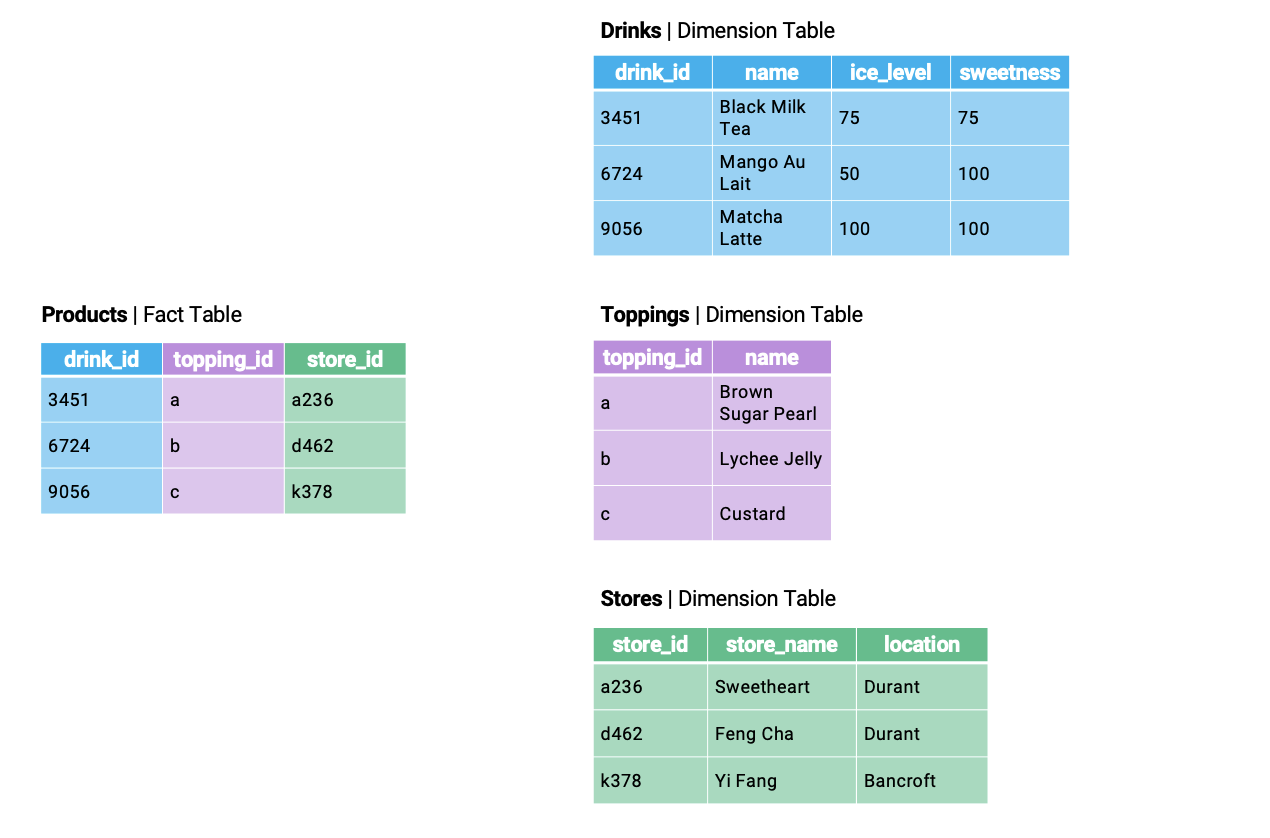
A common way of organizing a database is by using a star schema. A star schema is composed of two types of tables. A fact table is the central table of the database —— it contains the information needed to link entries across several dimension tables, which contain more detailed information about the data.

Say we were working with a database about boba offerings in Berkeley. The dimension tables of the database might contain information about tea varieties and boba toppings. The fact table would be used to link this information across the various dimension tables.

multidimensional

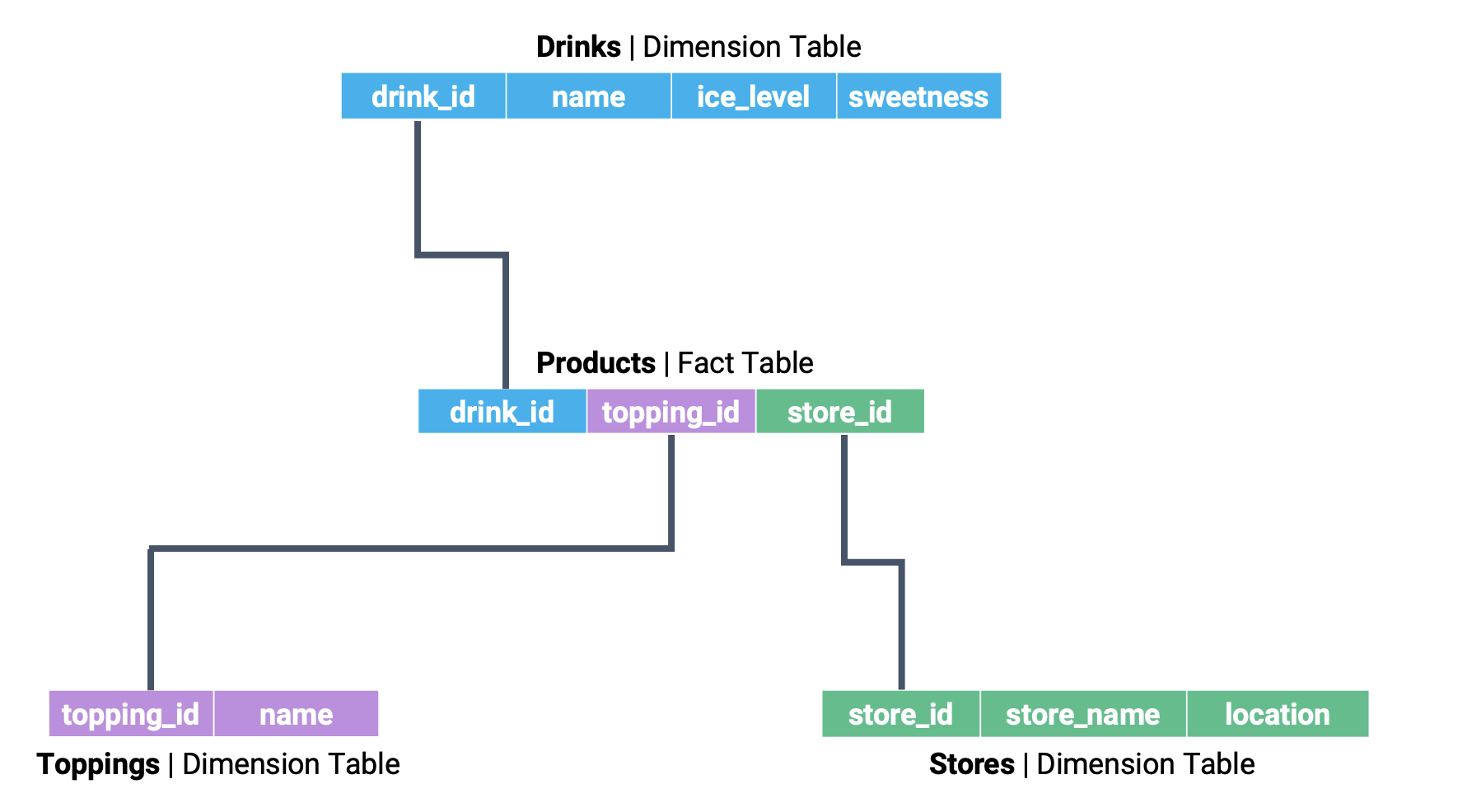
If we explicitly mark the relationships between tables, we start to see the star-like structure of the star schema.

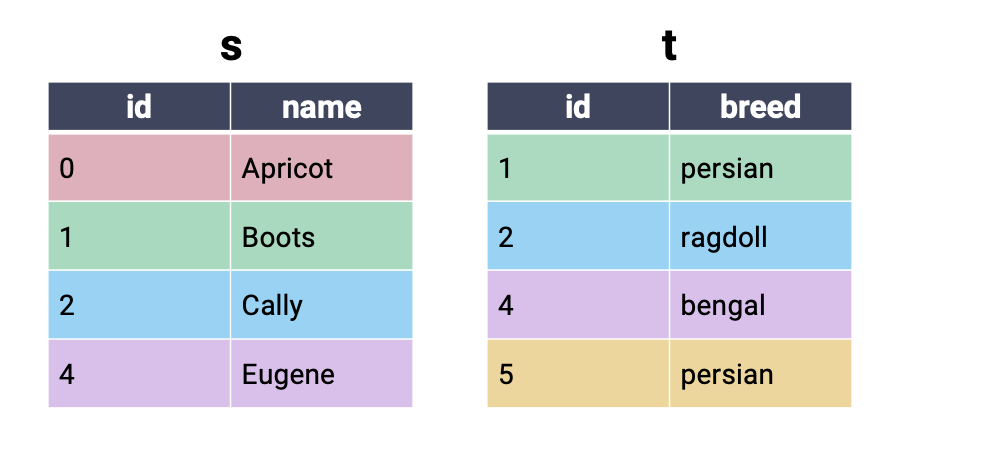
To join data across multiple tables, we’ll use the (creatively named) JOIN keyword. We’ll make things easier for now by first considering the simpler cats dataset, which consists of the tables s and t.

cats

To perform a join, we amend the FROM clause. You can think of this as saying, “SELECT my data FROM tables that have been JOINed together.”

Remember: SQL does not consider newlines or whitespace when interpreting queries. The indentation given in the example below is to help improve readability. If you wish, you can write code that does not follow this formatting.

SELECT <column list>
FROM table_1 
    JOIN table_2 
    ON key_1 = key_2;

We also need to specify what column from each table should be used to determine matching entries. By defining these keys, we provide SQL with the information it needs to pair rows of data together.

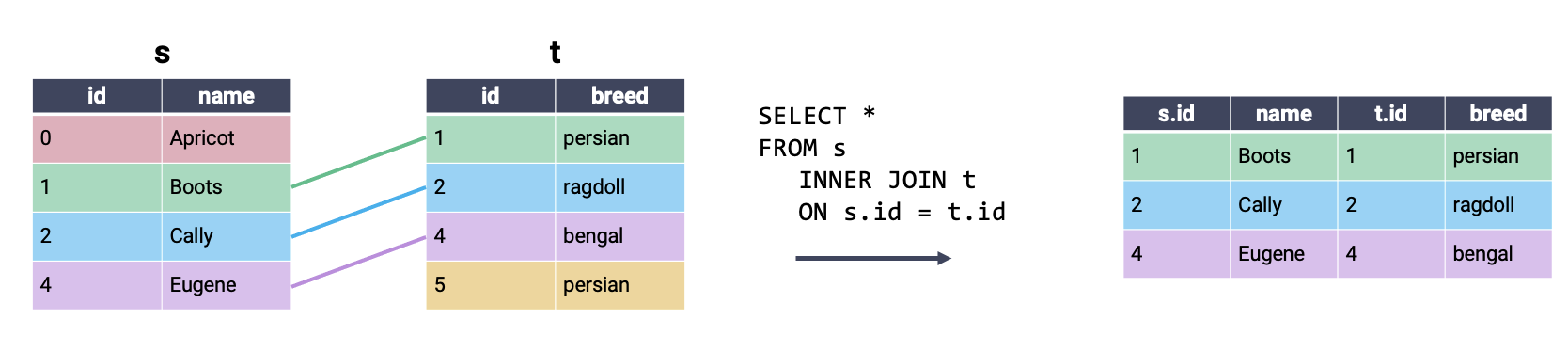
The most commonly used type of SQL JOIN is the inner join. It turns out you’re already familiar with what an inner join does, and how it works – this is the type of join we’ve been using in pandas all along! In an inner join, we combine every row in our first table with its matching entry in the second table. If a row from either table does not have a match in the other table, it is omitted from the output.

inner

In a cross join, all possible combinations of rows appear in the output table, regardless of whether or not rows share a matching key. Because all rows are joined, even if there is no matching key, it is not necessary to specify what keys to consider in an ON statement. A cross join is also known as a cartesian product.

cross

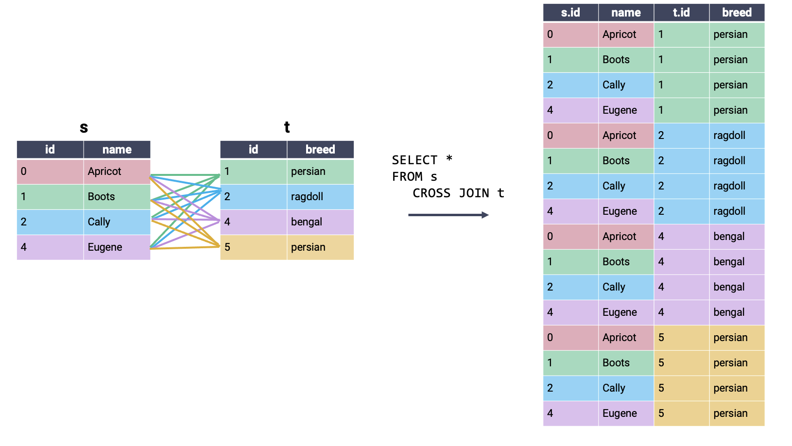
Conceptually, we can interpret an inner join as a cross join, followed by removing all rows that do not share a matching key. Notice that the output of the inner join above contains all rows of the cross join example that contain a single color across the entire row.

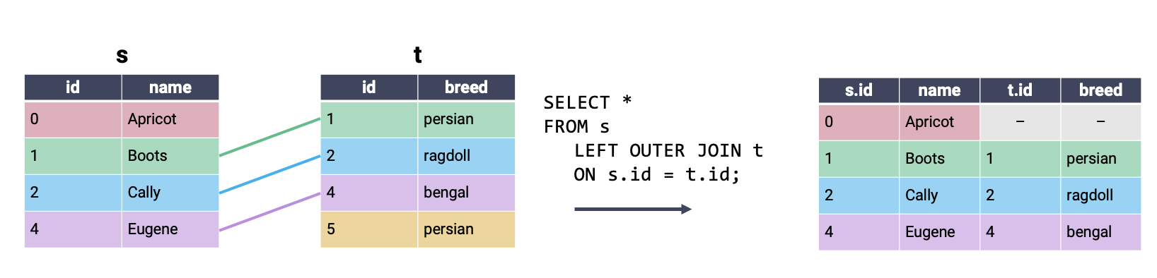
In a left outer join, all rows in the left table are kept in the output table. If a row in the right table shares a match with the left table, this row will be kept; otherwise, the rows in the right table are omitted from the output. We can fill in any missing values with NULL.

left

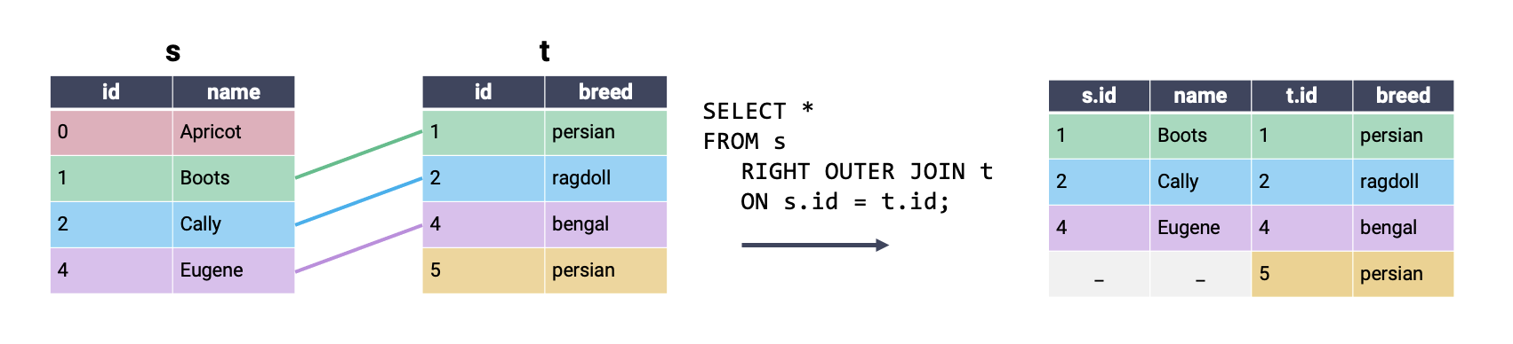
A right outer join keeps all rows in the right table. Rows in the left table are only kept if they share a match in the right table. Again, we can fill in any missing values with NULL.

right

In a full outer join, all rows that have a match between the two tables are joined together. If a row has no match in the second table, then the values of the columns for that second table are filled with NULL. In other words, a full outer join performs an inner join while still keeping rows that have no match in the other table. This is best understood visually:

full

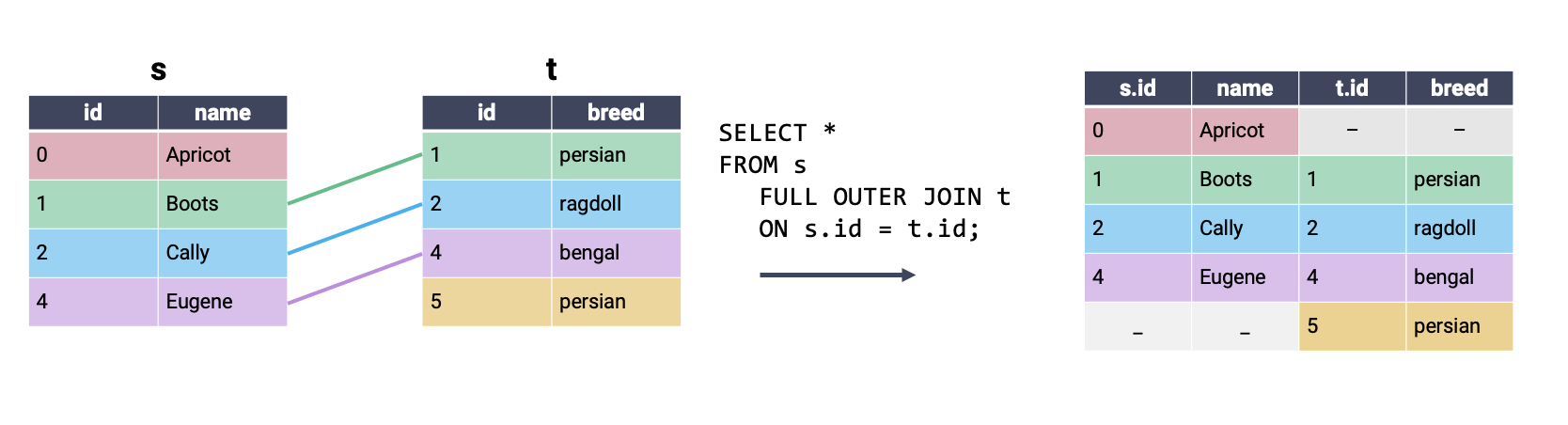
We have kept the same output achieved using an inner join, with the addition of partially null rows for entries in s and t that had no match in the second table.

21.5.1 Aliasing in `JOIN`s

When joining tables, we often create aliases for table names (similarly to what we did with column names in the last lecture). We do this as it is typically easier to refer to aliases, especially when we are working with long table names. We can even reference columns using aliased table names!

Let’s say we want to determine the average rating of various movies. We’ll need to JOIN the Title and Rating tables and can create aliases for both tables.

%%sql

SELECT primaryTitle, averageRating
FROM Title AS T INNER JOIN Rating AS R
ON T.tconst = R.tconst;

Running query in 'imdb'

primaryTitle	averageRating
Schwägereltern	4.599999904632568
IndeXovci: Izbori, jer ste vi to trazili	7.699999809265137
A Nightmare in Las Cruces: Part 2	3.0999999046325684
New York	8.199999809265137
Cha-lui: Lost in Seoul	4.699999809265137
Crazy Beautiful You	6.900000095367432
Saken	7.199999809265137
Rattle the Cage	6.599999904632568
To Dream	5.0
Cerca de tu casa	6.099999904632568

ResultSet : to convert to pandas, call .DataFrame() or to polars, call .PolarsDataFrame()
Truncated to displaylimit of 10
If you want to see more, please visit displaylimit configuration

Note that the AS is actually optional! We can create aliases for our tables even without it, but we usually include it for clarity.

%%sql

SELECT primaryTitle, averageRating
FROM Title T INNER JOIN Rating R
ON T.tconst = R.tconst;

Running query in 'imdb'

primaryTitle	averageRating
The Art of Cruising Men	5.599999904632568
Aventurero del mar	3.9000000953674316
The Beautiful Washing Machine	5.400000095367432
Hollywood, It's a Dog's Life	5.099999904632568
C(r)ook	6.300000190734863
Caballos en la ciudad	7.800000190734863
Calvaire	6.099999904632568
Skinny and Fatty	8.399999618530273
Chicks 101	7.099999904632568
Les cinéphiles 2 - Eric a disparu	5.300000190734863

ResultSet : to convert to pandas, call .DataFrame() or to polars, call .PolarsDataFrame()
Truncated to displaylimit of 10
If you want to see more, please visit displaylimit configuration

21.5.2 Common Table Expressions

For more sophisticated data problems, the queries can become very complex. Common table expressions (CTEs) allow us to break down these complex queries into more manageable parts. To do so, we create temporary tables corresponding to different aspects of the problem and then reference them in the final query:

WITH 
table_name1 AS ( 
    SELECT ...
),
table_name2 AS ( 
    SELECT ...
)
SELECT ... 
FROM 
table_name1, 
table_name2, ...

Let’s say we want to identify the top 10 action movies that are highly rated (with an average rating greater than 7) and popular (having more than 5000 votes), along with the primary actors who are the most popular. We can use CTEs to break this query down into separate problems. Initially, we can filter to find good action movies and prolific actors separately. This way, in our final join, we only need to change the order.

%%sql
WITH 
good_action_movies AS (
    SELECT *
    FROM Title T JOIN Rating R ON T.tconst = R.tconst  
    WHERE genres LIKE '%Action%' AND averageRating > 7 AND numVotes > 5000
),
prolific_actors AS (
    SELECT N.nconst, primaryName, COUNT(*) as numRoles
    FROM Name N JOIN Principal P ON N.nconst = P.nconst
    WHERE category = 'actor'
    GROUP BY N.nconst, primaryName
)
SELECT primaryTitle, primaryName, numRoles, ROUND(averageRating) AS rating
FROM good_action_movies m, prolific_actors a, principal p
WHERE p.tconst = m.tconst AND p.nconst = a.nconst
ORDER BY rating DESC, numRoles DESC
LIMIT 10;

Running query in 'imdb'

primaryTitle	primaryName	numRoles	rating
Threat Level Midnight: The Movie	Steve Carell	51	10.0
Threat Level Midnight: The Movie	Steve Carell	51	10.0
Threat Level Midnight: The Movie	Rainn Wilson	36	10.0
Threat Level Midnight: The Movie	Ed Helms	36	10.0
Threat Level Midnight: The Movie	Ed Helms	36	10.0
Threat Level Midnight: The Movie	John Krasinski	28	10.0
Threat Level Midnight: The Movie	Craig Robinson	26	10.0
Threat Level Midnight: The Movie	Ricky Gervais	17	10.0
Threat Level Midnight: The Movie	Stephen Merchant	14	10.0
Threat Level Midnight: The Movie	Creed Bratton	12	10.0

ResultSet : to convert to pandas, call .DataFrame() or to polars, call .PolarsDataFrame()
Truncated to displaylimit of 10
If you want to see more, please visit displaylimit configuration

21.1 Aggregating with GROUP BY

21.2 Filtering Groups

21.3 Summary: SQL

21.4 EDA in SQL

21.4.1 Matching Text using LIKE

21.4.2 CASTing Data Types

21.4.3 Using Conditional Statements with CASE

21.5 JOINing Tables

21.5.1 Aliasing in JOINs

21.5.2 Common Table Expressions

21.1 Aggregating with `GROUP BY`

21.4.1 Matching Text using `LIKE`

21.4.2 `CAST`ing Data Types

21.4.3 Using Conditional Statements with `CASE`

21.5 `JOIN`ing Tables

21.5.1 Aliasing in `JOIN`s