2 Pandas I

Learning Outcomes

Build familiarity with pandas and pandas syntax.
Learn key data structures: DataFrame, Series, and Index.
Understand methods for extracting data: .loc, .iloc, and [].

In this sequence of lectures, we will dive right into things by having you explore and manipulate real-world data. We’ll first introduce pandas, a popular Python library for interacting with tabular data.

2.1 Tabular Data

Data scientists work with data stored in a variety of formats. This class focuses primarily on tabular data — data that is stored in a table.

Tabular data is one of the most common systems that data scientists use to organize data. This is in large part due to the simplicity and flexibility of tables. Tables allow us to represent each observation, or instance of collecting data from an individual, as its own row. We can record each observation’s distinct characteristics, or features, in separate columns.

To see this in action, we’ll explore the elections dataset, which stores information about political candidates who ran for president of the United States in previous years.

In the elections dataset, each row (blue box) represents one instance of a candidate running for president in a particular year. For example, the first row represents Andrew Jackson running for president in the year 1824. Each column (yellow box) represents one characteristic piece of information about each presidential candidate. For example, the column named “Result” stores whether or not the candidate won the election.

Your work in Data 8 helped you grow very familiar with using and interpreting data stored in a tabular format. Back then, you used the Table class of the datascience library, a special programming library created specifically for Data 8 students.

In Data 100, we will be working with the programming library pandas, which is generally accepted in the data science community as the industry- and academia-standard tool for manipulating tabular data (as well as the inspiration for Petey, our panda bear mascot).

Using pandas, we can

Arrange data in a tabular format.
Extract useful information filtered by specific conditions.
Operate on data to gain new insights.
Apply NumPy functions to our data (our friends from Data 8).
Perform vectorized computations to speed up our analysis (Lab 1).

2.2 `Series`, `DataFrame`s, and Indices

To begin our work in pandas, we must first import the library into our Python environment. This will allow us to use pandas data structures and methods in our code.

# `pd` is the conventional alias for Pandas, as `np` is for NumPy
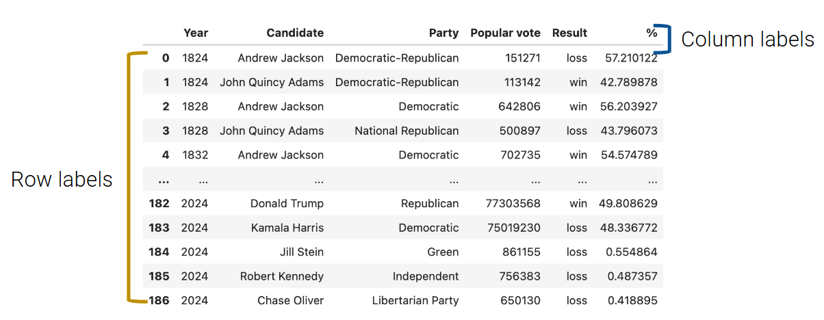
import pandas as pd

There are three fundamental data structures in pandas:

Series: 1D labeled array data; best thought of as columnar data.
DataFrame: 2D tabular data with rows and columns.
Index: A sequence of row/column labels.

DataFrames, Series, and Indices can be represented visually in the following diagram, which considers the first few rows of the elections dataset.

Notice how the DataFrame is a two-dimensional object — it contains both rows and columns. The Series above is a singular column of this DataFrame, namely the Result column. Both contain an Index, or a shared list of row labels (the integers from 0 to 4, inclusive).

2.2.1 Series

A Series represents a column of a DataFrame; more generally, it can be any 1-dimensional array-like object. It contains both:

A sequence of values of the same type.
A sequence of data labels called the index.

In the cell below, we create a Series named s.

s = pd.Series(["welcome", "to", "data 100"])
s

0     welcome
1          to
2    data 100
dtype: object

 # Accessing data values within the Series
 s.values

array(['welcome', 'to', 'data 100'], dtype=object)

 # Accessing the Index of the Series
 s.index

RangeIndex(start=0, stop=3, step=1)

By default, the index of a Series is a sequential list of integers beginning from 0. Optionally, a manually specified list of desired indices can be passed to the index argument.

s = pd.Series([-1, 10, 2], index = ["a", "b", "c"])
s

a    -1
b    10
c     2
dtype: int64

s.index

Index(['a', 'b', 'c'], dtype='object')

Indices can also be changed after initialization.

s.index = ["first", "second", "third"]
s

first     -1
second    10
third      2
dtype: int64

s.index

Index(['first', 'second', 'third'], dtype='object')

2.2.1.1 Selection in `Series`

Much like when working with NumPy arrays, we can select a single value or a set of values from a Series. To do so, there are three primary methods:

A single label.
A list of labels.
A filtering condition.

To demonstrate this, let’s define a new Series s.

s = pd.Series([4, -2, 0, 6], index = ["a", "b", "c", "d"])
s

a    4
b   -2
c    0
d    6
dtype: int64

2.2.1.1.1 A Single Label

# We return the value stored at the index label "a"
s["a"]

np.int64(4)

2.2.1.1.2 A List of Labels

# We return a Series of the values stored at the index labels "a" and "c"
s[["a", "c"]]

a    4
c    0
dtype: int64

2.2.1.1.3 A Filtering Condition

Perhaps the most interesting (and useful) method of selecting data from a Series is by using a filtering condition.

First, we apply a boolean operation to the Series. This creates a new Series of boolean values.

# Filter condition: select all elements greater than 0
s > 0

a     True
b    False
c    False
d     True
dtype: bool

We then use this boolean condition to index into our original Series. pandas will select only the entries in the original Series that satisfy the condition.

s[s > 0]

a    4
d    6
dtype: int64

2.2.2 `DataFrames`

Typically, we will work with Series using the perspective that they are columns in a DataFrame. We can think of a DataFrame as a collection of Series that all share the same Index.

In Data 8, you encountered the Table class of the datascience library, which represented tabular data. In Data 100, we’ll be using the DataFrame class of the pandas library.

2.2.2.1 Creating a `DataFrame`

There are many ways to create a DataFrame. Here, we will cover the most popular approaches:

From a CSV file.
Using a list and column name(s).
From a dictionary.
From a Series.

More generally, the syntax for creating a DataFrame is:

 pandas.DataFrame(data, index, columns)

2.2.2.1.1 From a CSV file

In Data 100, our data are typically stored in a CSV (comma-separated values) file format. We can import a CSV file into a DataFrame by passing the data path as an argument to the following pandas function.
pd.read_csv("filename.csv")

With our new understanding of pandas in hand, let’s return to the elections dataset from before. Now, we can recognize that it is represented as a pandas DataFrame.

elections = pd.read_csv("data/elections.csv")
elections

	Year	Candidate	Party	Popular vote	Result	%
0	1824	Andrew Jackson	Democratic-Republican	151271	loss	57.210122
1	1824	John Quincy Adams	Democratic-Republican	113142	win	42.789878
2	1828	Andrew Jackson	Democratic	642806	win	56.203927
3	1828	John Quincy Adams	National Republican	500897	loss	43.796073
4	1832	Andrew Jackson	Democratic	702735	win	54.574789
...	...	...	...	...	...	...
182	2024	Donald Trump	Republican	77303568	win	49.808629
183	2024	Kamala Harris	Democratic	75019230	loss	48.336772
184	2024	Jill Stein	Green	861155	loss	0.554864
185	2024	Robert Kennedy	Independent	756383	loss	0.487357
186	2024	Chase Oliver	Libertarian Party	650130	loss	0.418895

187 rows × 6 columns

This code stores our DataFrame object in the elections variable. Upon inspection, our elections DataFrame has 182 rows and 6 columns (Year, Candidate, Party, Popular Vote, Result, %). Each row represents a single record — in our example, a presidential candidate from some particular year. Each column represents a single attribute or feature of the record.

2.2.2.1.2 Using a List and Column Name(s)

We’ll now explore creating a DataFrame with data of our own.

Consider the following examples. The first code cell creates a DataFrame with a single column Numbers.

df_list = pd.DataFrame([1, 2, 3], columns=["Numbers"])
df_list

	Numbers
0	1
1	2
2	3

The second creates a DataFrame with the columns Numbers and Description. Notice how a 2D list of values is required to initialize the second DataFrame — each nested list represents a single row of data.

df_list = pd.DataFrame([[1, "one"], [2, "two"]], columns = ["Number", "Description"])
df_list

	Number	Description
0	1	one
1	2	two

2.2.2.1.3 From a Dictionary

A third (and more common) way to create a DataFrame is with a dictionary. The dictionary keys represent the column names, and the dictionary values represent the column values.

Below are two ways of implementing this approach. The first is based on specifying the columns of the DataFrame, whereas the second is based on specifying the rows of the DataFrame.

df_dict = pd.DataFrame({
    "Fruit": ["Strawberry", "Orange"], 
    "Price": [5.49, 3.99]
})
df_dict

	Fruit	Price
0	Strawberry	5.49
1	Orange	3.99

df_dict = pd.DataFrame(
    [
        {"Fruit":"Strawberry", "Price":5.49}, 
        {"Fruit": "Orange", "Price":3.99}
    ]
)
df_dict

	Fruit	Price
0	Strawberry	5.49
1	Orange	3.99

2.2.2.1.4 From a `Series`

Earlier, we explained how a Series was synonymous to a column in a DataFrame. It follows, then, that a DataFrame is equivalent to a collection of Series, which all share the same Index.

In fact, we can initialize a DataFrame by merging two or more Series. Consider the Series s_a and s_b.

# Notice how our indices, or row labels, are the same

s_a = pd.Series(["a1", "a2", "a3"], index = ["r1", "r2", "r3"])
s_b = pd.Series(["b1", "b2", "b3"], index = ["r1", "r2", "r3"])

We can turn individual Series into a DataFrame using two common methods (shown below):

pd.DataFrame(s_a)

	0
r1	a1
r2	a2
r3	a3

s_b.to_frame()

	0
r1	b1
r2	b2
r3	b3

To merge the two Series and specify their column names, we use the following syntax:

pd.DataFrame({
    "A-column": s_a, 
    "B-column": s_b
})

	A-column	B-column
r1	a1	b1
r2	a2	b2
r3	a3	b3

2.2.3 Indices

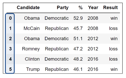
On a more technical note, an index doesn’t have to be an integer, nor does it have to be unique. For example, we can set the index of the elections DataFrame to be the name of presidential candidates.

# Creating a DataFrame from a CSV file and specifying the index column
elections = pd.read_csv("data/elections.csv", index_col = "Candidate")
elections

	Year	Party	Popular vote	Result	%
Candidate
Andrew Jackson	1824	Democratic-Republican	151271	loss	57.210122
John Quincy Adams	1824	Democratic-Republican	113142	win	42.789878
Andrew Jackson	1828	Democratic	642806	win	56.203927
John Quincy Adams	1828	National Republican	500897	loss	43.796073
Andrew Jackson	1832	Democratic	702735	win	54.574789
...	...	...	...	...	...
Donald Trump	2024	Republican	77303568	win	49.808629
Kamala Harris	2024	Democratic	75019230	loss	48.336772
Jill Stein	2024	Green	861155	loss	0.554864
Robert Kennedy	2024	Independent	756383	loss	0.487357
Chase Oliver	2024	Libertarian Party	650130	loss	0.418895

187 rows × 5 columns

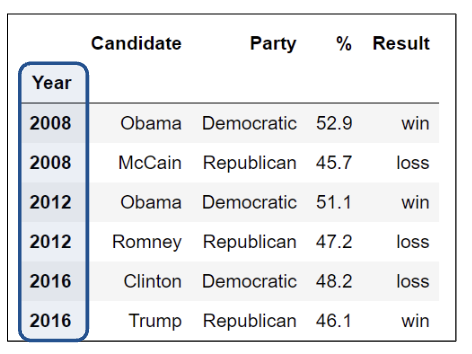
We can also select a new column and set it as the index of the DataFrame. For example, we can set the index of the elections DataFrame to represent the candidate’s party.

elections.reset_index(inplace = True) # Resetting the index so we can set it again
# This sets the index to the "Party" column
elections.set_index("Party")

	Candidate	Year	Popular vote	Result	%
Party
Democratic-Republican	Andrew Jackson	1824	151271	loss	57.210122
Democratic-Republican	John Quincy Adams	1824	113142	win	42.789878
Democratic	Andrew Jackson	1828	642806	win	56.203927
National Republican	John Quincy Adams	1828	500897	loss	43.796073
Democratic	Andrew Jackson	1832	702735	win	54.574789
...	...	...	...	...	...
Republican	Donald Trump	2024	77303568	win	49.808629
Democratic	Kamala Harris	2024	75019230	loss	48.336772
Green	Jill Stein	2024	861155	loss	0.554864
Independent	Robert Kennedy	2024	756383	loss	0.487357
Libertarian Party	Chase Oliver	2024	650130	loss	0.418895

187 rows × 5 columns

And, if we’d like, we can revert the index back to the default list of integers.

# This resets the index to be the default list of integer
elections.reset_index(inplace=True) 
elections.index

RangeIndex(start=0, stop=187, step=1)

It is also important to note that the row labels that constitute an index don’t have to be unique. While index values can be unique and numeric, acting as a row number, they can also be named and non-unique.

Here we see unique and numeric index values.

However, here the index values are not unique.

2.3 `DataFrame` Attributes: Index, Columns, and Shape

On the other hand, column names in a DataFrame are almost always unique. Looking back to the elections dataset, it wouldn’t make sense to have two columns named "Candidate". Sometimes, you’ll want to extract these different values, in particular, the list of row and column labels.

For index/row labels, use DataFrame.index:

elections.set_index("Party", inplace = True)
elections.index

Index(['Democratic-Republican', 'Democratic-Republican', 'Democratic',
       'National Republican', 'Democratic', 'National Republican',
       'Anti-Masonic', 'Whig', 'Democratic', 'Whig',
       ...
       'Green', 'Democratic', 'Republican', 'Libertarian', 'Green',
       'Republican', 'Democratic', 'Green', 'Independent',
       'Libertarian Party'],
      dtype='object', name='Party', length=187)

For column labels, use DataFrame.columns:

elections.columns

Index(['index', 'Candidate', 'Year', 'Popular vote', 'Result', '%'], dtype='object')

And for the shape of the DataFrame, we can use DataFrame.shape to get the number of rows followed by the number of columns:

elections.shape

(187, 6)

2.4 Slicing in `DataFrame`s

Now that we’ve learned more about DataFrames, let’s dive deeper into their capabilities.

The API (Application Programming Interface) for the DataFrame class is enormous. In this section, we’ll discuss several methods of the DataFrame API that allow us to extract subsets of data.

The simplest way to manipulate a DataFrame is to extract a subset of rows and columns, known as slicing.

Common ways we may want to extract data are grabbing:

The first or last n rows in the DataFrame.
Data with a certain label.
Data at a certain position.

We will do so with four primary methods of the DataFrame class:

.head and .tail
.loc
.iloc
[]

2.4.1 Extracting data with `.head` and `.tail`

The simplest scenario in which we want to extract data is when we simply want to select the first or last few rows of the DataFrame.

To extract the first n rows of a DataFrame df, we use the syntax df.head(n).

Code

elections = pd.read_csv("data/elections.csv")

# Extract the first 5 rows of the DataFrame
elections.head(5)

	Year	Candidate	Party	Popular vote	Result	%
0	1824	Andrew Jackson	Democratic-Republican	151271	loss	57.210122
1	1824	John Quincy Adams	Democratic-Republican	113142	win	42.789878
2	1828	Andrew Jackson	Democratic	642806	win	56.203927
3	1828	John Quincy Adams	National Republican	500897	loss	43.796073
4	1832	Andrew Jackson	Democratic	702735	win	54.574789

Similarly, calling df.tail(n) allows us to extract the last n rows of the DataFrame.

# Extract the last 5 rows of the DataFrame
elections.tail(5)

	Year	Candidate	Party	Popular vote	Result	%
182	2024	Donald Trump	Republican	77303568	win	49.808629
183	2024	Kamala Harris	Democratic	75019230	loss	48.336772
184	2024	Jill Stein	Green	861155	loss	0.554864
185	2024	Robert Kennedy	Independent	756383	loss	0.487357
186	2024	Chase Oliver	Libertarian Party	650130	loss	0.418895

2.4.2 Label-based Extraction: Indexing with `.loc`

For the more complex task of extracting data with specific column or index labels, we can use .loc. The .loc accessor allows us to specify the labels of rows and columns we wish to extract. The labels (commonly referred to as the indices) are the bold text on the far left of a DataFrame, while the column labels are the column names found at the top of a DataFrame.

To grab data with .loc, we must specify the row and column label(s) where the data exists. The row labels are the first argument to the .loc function; the column labels are the second.

Arguments to .loc can be:

A single value.
A slice.
A list.

For example, to select a single value, we can select the row labeled 0 and the column labeled Candidate from the elections DataFrame.

elections.loc[0, 'Candidate']

'Andrew Jackson'

Keep in mind that passing in just one argument as a single value will produce a Series. Below, we’ve extracted a subset of the "Popular vote" column as a Series.

elections.loc[[87, 25, 179], "Popular vote"]

87     15761254
25       848019
179    74216154
Name: Popular vote, dtype: int64

Note that if we pass "Popular vote" as a list, the output will be a DataFrame.

elections.loc[[87, 25, 179], ["Popular vote"]]

	Popular vote
87	15761254
25	848019
179	74216154

To select multiple rows and columns, we can use Python slice notation. Here, we select the rows from labels 0 to 3 and the columns from labels "Year" to "Popular vote". Notice that unlike Python slicing, .loc is inclusive of the right upper bound.

elections.loc[0:3, 'Year':'Popular vote']

	Year	Candidate	Party	Popular vote
0	1824	Andrew Jackson	Democratic-Republican	151271
1	1824	John Quincy Adams	Democratic-Republican	113142
2	1828	Andrew Jackson	Democratic	642806
3	1828	John Quincy Adams	National Republican	500897

Suppose that instead, we want to extract all column values for the first four rows in the elections DataFrame. The shorthand : is useful for this.

elections.loc[0:3, :]

	Year	Candidate	Party	Popular vote	Result	%
0	1824	Andrew Jackson	Democratic-Republican	151271	loss	57.210122
1	1824	John Quincy Adams	Democratic-Republican	113142	win	42.789878
2	1828	Andrew Jackson	Democratic	642806	win	56.203927
3	1828	John Quincy Adams	National Republican	500897	loss	43.796073

We can use the same shorthand to extract all rows.

elections.loc[:, ["Year", "Candidate", "Result"]]

	Year	Candidate	Result
0	1824	Andrew Jackson	loss
1	1824	John Quincy Adams	win
2	1828	Andrew Jackson	win
3	1828	John Quincy Adams	loss
4	1832	Andrew Jackson	win
...	...	...	...
182	2024	Donald Trump	win
183	2024	Kamala Harris	loss
184	2024	Jill Stein	loss
185	2024	Robert Kennedy	loss
186	2024	Chase Oliver	loss

187 rows × 3 columns

There are a couple of things we should note. Firstly, unlike conventional Python, pandas allows us to slice string values (in our example, the column labels). Secondly, slicing with .loc is inclusive. Notice how our resulting DataFrame includes every row and column between and including the slice labels we specified.

Equivalently, we can use a list to obtain multiple rows and columns in our elections DataFrame.

elections.loc[[0, 1, 2, 3], ['Year', 'Candidate', 'Party', 'Popular vote']]

	Year	Candidate	Party	Popular vote
0	1824	Andrew Jackson	Democratic-Republican	151271
1	1824	John Quincy Adams	Democratic-Republican	113142
2	1828	Andrew Jackson	Democratic	642806
3	1828	John Quincy Adams	National Republican	500897

Lastly, we can interchange list and slicing notation.

elections.loc[[0, 1, 2, 3], :]

	Year	Candidate	Party	Popular vote	Result	%
0	1824	Andrew Jackson	Democratic-Republican	151271	loss	57.210122
1	1824	John Quincy Adams	Democratic-Republican	113142	win	42.789878
2	1828	Andrew Jackson	Democratic	642806	win	56.203927
3	1828	John Quincy Adams	National Republican	500897	loss	43.796073

2.4.3 Integer-based Extraction: Indexing with `.iloc`

Slicing with .iloc works similarly to .loc. However, .iloc uses the index positions of rows and columns rather than the labels (think to yourself: loc uses lables; iloc uses indices). The arguments to the .iloc function also behave similarly — single values, lists, indices, and any combination of these are permitted.

Let’s begin reproducing our results from above. We’ll begin by selecting the first presidential candidate in our elections DataFrame:

# elections.loc[0, "Candidate"] - Previous approach
elections.iloc[0, 1]

'Andrew Jackson'

Notice how the first argument to both .loc and .iloc are the same. This is because the row with a label of 0 is conveniently in the \(0^{\text{th}}\) (equivalently, the first position) of the elections DataFrame. Generally, this is true of any DataFrame where the row labels are incremented in ascending order from 0.

And, as before, if we were to pass in only one single value argument, our result would be a Series.

elections.iloc[[1,2,3],1]

1    John Quincy Adams
2       Andrew Jackson
3    John Quincy Adams
Name: Candidate, dtype: object

However, when we select the first four rows and columns using .iloc, we notice something.

# elections.loc[0:3, 'Year':'Popular vote'] - Previous approach
elections.iloc[0:4, 0:4]

	Year	Candidate	Party	Popular vote
0	1824	Andrew Jackson	Democratic-Republican	151271
1	1824	John Quincy Adams	Democratic-Republican	113142
2	1828	Andrew Jackson	Democratic	642806
3	1828	John Quincy Adams	National Republican	500897

Slicing is no longer inclusive in .iloc — it’s exclusive. In other words, the right end of a slice is not included when using .iloc. This is one of the subtleties of pandas syntax; you will get used to it with practice.

List behavior works just as expected.

#elections.loc[[0, 1, 2, 3], ['Year', 'Candidate', 'Party', 'Popular vote']] - Previous Approach
elections.iloc[[0, 1, 2, 3], [0, 1, 2, 3]]

	Year	Candidate	Party	Popular vote
0	1824	Andrew Jackson	Democratic-Republican	151271
1	1824	John Quincy Adams	Democratic-Republican	113142
2	1828	Andrew Jackson	Democratic	642806
3	1828	John Quincy Adams	National Republican	500897

And just like with .loc, we can use a colon with .iloc to extract all rows or columns.

elections.iloc[:, 0:3]

	Year	Candidate	Party
0	1824	Andrew Jackson	Democratic-Republican
1	1824	John Quincy Adams	Democratic-Republican
2	1828	Andrew Jackson	Democratic
3	1828	John Quincy Adams	National Republican
4	1832	Andrew Jackson	Democratic
...	...	...	...
182	2024	Donald Trump	Republican
183	2024	Kamala Harris	Democratic
184	2024	Jill Stein	Green
185	2024	Robert Kennedy	Independent
186	2024	Chase Oliver	Libertarian Party

187 rows × 3 columns

This discussion begs the question: when should we use .loc vs. .iloc? In most cases, .loc is generally safer to use. You can imagine .iloc may return incorrect values when applied to a dataset where the ordering of data can change. However, .iloc can still be useful — for example, if you are looking at a DataFrame of sorted movie earnings and want to get the median earnings for a given year, you can use .iloc to index into the middle.

Overall, it is important to remember that:

.loc performances label-based extraction.
.iloc performs integer-based extraction.

2.4.4 Context-dependent Extraction: Indexing with `[]`

The [] selection operator is the most baffling of all, yet the most commonly used. It only takes a single argument, which may be one of the following:

A slice of row numbers.
A list of column labels.
A single-column label.

That is, [] is context-dependent. Let’s see some examples.

2.4.4.1 A slice of row numbers

Say we wanted the first four rows of our elections DataFrame.

elections[0:4]

	Year	Candidate	Party	Popular vote	Result	%
0	1824	Andrew Jackson	Democratic-Republican	151271	loss	57.210122
1	1824	John Quincy Adams	Democratic-Republican	113142	win	42.789878
2	1828	Andrew Jackson	Democratic	642806	win	56.203927
3	1828	John Quincy Adams	National Republican	500897	loss	43.796073

2.4.4.2 A list of column labels

Suppose we now want the first four columns.

elections[["Year", "Candidate", "Party", "Popular vote"]]

	Year	Candidate	Party	Popular vote
0	1824	Andrew Jackson	Democratic-Republican	151271
1	1824	John Quincy Adams	Democratic-Republican	113142
2	1828	Andrew Jackson	Democratic	642806
3	1828	John Quincy Adams	National Republican	500897
4	1832	Andrew Jackson	Democratic	702735
...	...	...	...	...
182	2024	Donald Trump	Republican	77303568
183	2024	Kamala Harris	Democratic	75019230
184	2024	Jill Stein	Green	861155
185	2024	Robert Kennedy	Independent	756383
186	2024	Chase Oliver	Libertarian Party	650130

187 rows × 4 columns

2.4.4.3 A single-column label

Lastly, [] allows us to extract only the "Candidate" column.

elections["Candidate"]

0         Andrew Jackson
1      John Quincy Adams
2         Andrew Jackson
3      John Quincy Adams
4         Andrew Jackson
             ...        
182         Donald Trump
183        Kamala Harris
184           Jill Stein
185       Robert Kennedy
186         Chase Oliver
Name: Candidate, Length: 187, dtype: object

The output is a Series! In this course, we’ll become very comfortable with [], especially for selecting columns. In practice, [] is much more common than .loc, especially since it is far more concise.

2.5 Parting Note

The pandas library is enormous and contains many useful functions. Here is a link to its documentation. We certainly don’t expect you to memorize each and every method of the library, and we will give you a reference sheet for exams.

The introductory Data 100 pandas lectures will provide a high-level view of the key data structures and methods that will form the foundation of your pandas knowledge. A goal of this course is to help you build your familiarity with the real-world programming practice of … Googling! Answers to your questions can be found in documentation, Stack Overflow, etc. Being able to search for, read, and implement documentation is an important life skill for any data scientist.

With that, we will move on to Pandas II!

2.1 Tabular Data

2.2 Series, DataFrames, and Indices

2.2.1 Series

2.2.1.1 Selection in Series

2.2.1.1.1 A Single Label

2.2.1.1.2 A List of Labels

2.2.1.1.3 A Filtering Condition

2.2.2 DataFrames

2.2.2.1 Creating a DataFrame

2.2.2.1.1 From a CSV file

2.2.2.1.2 Using a List and Column Name(s)

2.2.2.1.3 From a Dictionary

2.2.2.1.4 From a Series

2.2.3 Indices

2.3 DataFrame Attributes: Index, Columns, and Shape

2.4 Slicing in DataFrames

2.4.1 Extracting data with .head and .tail

2.4.2 Label-based Extraction: Indexing with .loc

2.4.3 Integer-based Extraction: Indexing with .iloc

2.4.4 Context-dependent Extraction: Indexing with []

2.4.4.1 A slice of row numbers

2.4.4.2 A list of column labels

2.4.4.3 A single-column label

2.5 Parting Note

2.2 `Series`, `DataFrame`s, and Indices

2.2.1.1 Selection in `Series`

2.2.2 `DataFrames`

2.2.2.1 Creating a `DataFrame`

2.2.2.1.4 From a `Series`

2.3 `DataFrame` Attributes: Index, Columns, and Shape

2.4 Slicing in `DataFrame`s

2.4.1 Extracting data with `.head` and `.tail`

2.4.2 Label-based Extraction: Indexing with `.loc`

2.4.3 Integer-based Extraction: Indexing with `.iloc`

2.4.4 Context-dependent Extraction: Indexing with `[]`