Code
import pandas as pd
import numpy as np
import scipy as sp
import plotly.express as px
import seaborn as snsSo far in this course, we’ve focused on supervised learning techniques that create a function to map inputs (features) to labelled outputs. Regression and classification are two main examples, where the output value of regression is quantitative while the output value of classification is categorical.
Today, we’ll introduce an unsupervised learning technique called PCA. Unlike supervised learning, unsupervised learning is applied to unlabeled data. Because we have features but no labels, we aim to identify patterns in those features. Principal Component Analysis (PCA) is a linear technique for dimensionality reduction, and PCA relies on a linear algebra algorithm called Singular Value Decomposition, which we will discuss more in the next lecture.
Visualization can help us identify clusters or patterns in our dataset, and it can give us an intuition about our data and how to clean it for the model. For this demo, we’ll return to the MPG dataset from Lecture 19 and see how far we can push visualization for multiple features.
import pandas as pd
import numpy as np
import scipy as sp
import plotly.express as px
import seaborn as snsmpg = sns.load_dataset("mpg").dropna()
mpg.head()| mpg | cylinders | displacement | horsepower | weight | acceleration | model_year | origin | name | |
|---|---|---|---|---|---|---|---|---|---|
| 0 | 18.0 | 8 | 307.0 | 130.0 | 3504 | 12.0 | 70 | usa | chevrolet chevelle malibu |
| 1 | 15.0 | 8 | 350.0 | 165.0 | 3693 | 11.5 | 70 | usa | buick skylark 320 |
| 2 | 18.0 | 8 | 318.0 | 150.0 | 3436 | 11.0 | 70 | usa | plymouth satellite |
| 3 | 16.0 | 8 | 304.0 | 150.0 | 3433 | 12.0 | 70 | usa | amc rebel sst |
| 4 | 17.0 | 8 | 302.0 | 140.0 | 3449 | 10.5 | 70 | usa | ford torino |
We can plot one feature as a histogram to see it’s distribution. Since we only plot one feature, we consider this a 1-dimensional plot.
px.histogram(mpg, x="displacement")We can also visualize two features (2-dimensional scatter plot):
px.scatter(mpg, x="displacement", y="horsepower")Three features (3-dimensional scatter plot):
fig = px.scatter_3d(mpg, x="displacement", y="horsepower", z="weight",
                    width=800, height=800)
fig.update_traces(marker=dict(size=3))
We can even push to 4 features using a 3D scatter plot and a colorbar:
fig = px.scatter_3d(mpg, x="displacement",
                    y="horsepower",
                    z="weight",
                    color="model_year",
                    width=800, height=800,
                    opacity=.7)
fig.update_traces(marker=dict(size=5))
Visualizing 5 features is also possible if we make the scatter dots unique to the datapoint’s origin.
fig = px.scatter_3d(mpg, x="displacement",
                    y="horsepower",
                    z="weight",
                    color="model_year",
                    size="mpg",
                    symbol="origin",
                    width=900, height=800,
                    opacity=.7)
# hide color scale legend on the plotly fig
fig.update_layout(coloraxis_showscale=False)
However, adding more features to our visualization can make our plot look messy and uninformative, and it can also be near impossible if we have a large number of features. The problem is that many datasets come with more than 5 features — hundreds, even. Is it still possible to visualize all those features?
Suppose we have a dataset of:
Let’s “rename” this in terms of linear algebra so that we can be more clear with our wording. Using linear algebra, we can view our matrix as:
The intrinsic dimension of a dataset is the minimal set of dimensions needed to approximately represent the data. In linear algebra terms, it is the dimension of the column space of a matrix, or the number of linearly independent columns in a matrix; this is equivalently called the rank of a matrix.
In the examples below, Dataset 1 has 2 dimensions because it has 2 linearly independent columns. Similarly, Dataset 2 has 3 dimensions because it has 3 linearly independent columns.
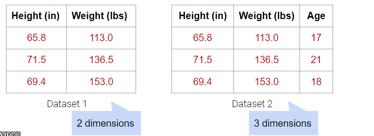
What about Dataset 4 below?
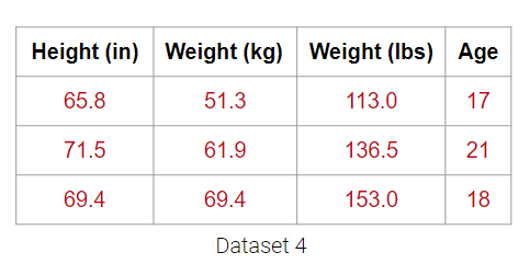
It may be tempting to say that it has 4 dimensions, but the Weight (lbs) column is actually just a linear transformation of the Weight (kg) column. Thus, no new information is captured, and the matrix of our dataset has a (column) rank of 3! Therefore, despite having 4 columns, we still say that this data is 3-dimensional.
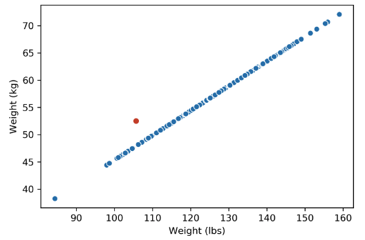
Plotting the weight columns together reveals the key visual intuition. While the two columns visually span a 2D space as a line, the data does not deviate at all from that singular line. This means that one of the weight columns is redundant! Even given the option to cover the whole 2D space, the data below does not. It might as well not have this dimension, which is why we still do not consider the data below to span more than 1 dimension.

What happens when there are outliers? Below, we’ve added one outlier point to the dataset above, and just that one point is enough to change the rank of the matrix from 1 to 2 dimensions. However, the data is still approximately 1-dimensional.
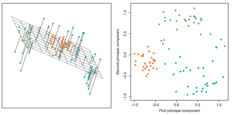
Dimensionality reduction is generally an approximation of the original data that’s achieved through matrix decomposition by projecting the data onto a desired dimension. In the example below, our original datapoints (blue dots) are 2-dimensional. We have a few choices if we want to project them down to 1-dimension: project them onto the \(x\)-axis (left), project them onto the \(y\)-axis (middle), or project them to a line \(mx + b\) (right). The resulting datapoints after the projection is shown in red. Which projection do you think is better? How can we calculate that?
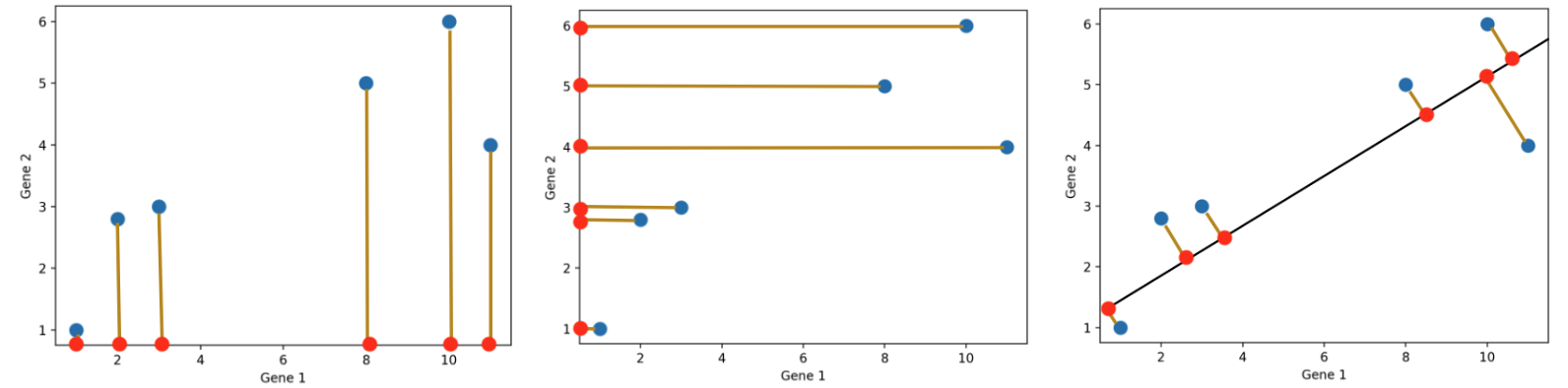
In general, we want the projection which is the best approximation for the original data (the graph on the right). In other words, we want the projection that captures the most variance of the original data. In the next section, we’ll see how this is calculated.
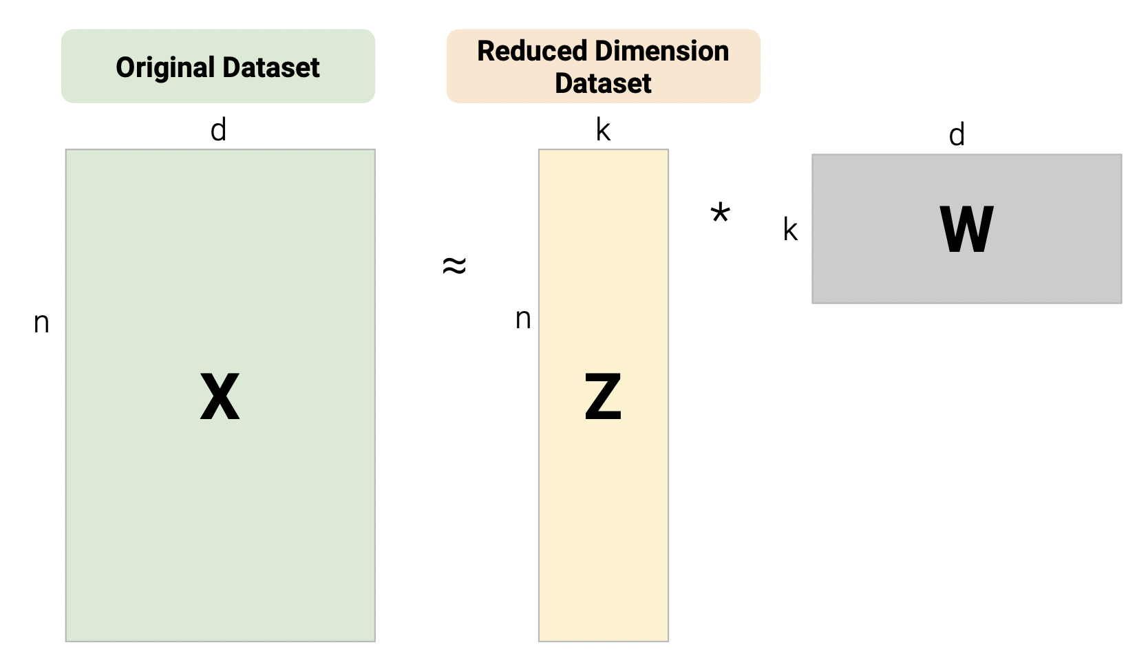
One linear technique for dimensionality reduction is matrix decomposition, which is closely tied to matrix multiplication. In this section, we will decompose our data matrix \(X\) into a lower-dimensional matrix \(Z\) that approximately recovers the original data when multiplied by \(W\).
First, consider the matrix multiplication example below:
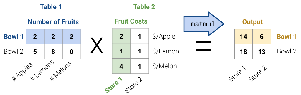
In general, there are two ways to interpret matrix multiplication:
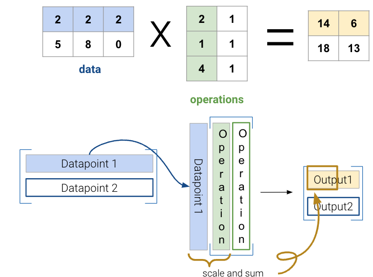
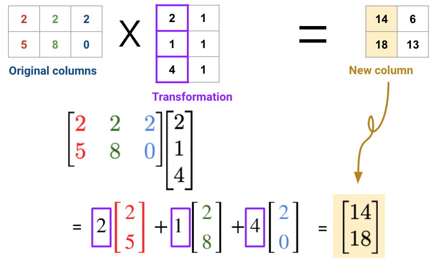
We will use the second interpretation to link matrix multiplication with matrix decomposition, where we receive a lower dimensional representation of data along with a transformation matrix.
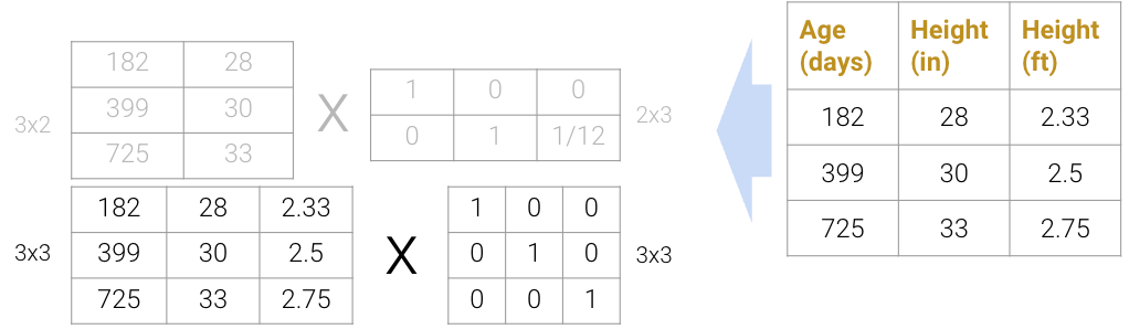
Matrix decomposition (a.k.a matrix factorization) is the opposite of matrix multiplication. Instead of multiplying two matrices, we want to decompose a single matrix into 2 separate matrices. Just like with real numbers, there are infinite ways to decompose a matrix into a product of two matrices. For example, \(9.9\) can be decomposed as \(1.1 * 9\), \(3.3 * 3\), \(1 * 9.9\), etc. Additionally, the sizes of the 2 decomposed matrices can vary drastically. In the example below, the first factorization (top) multiplies a \(3\times2\) matrix by a \(2\times3\) matrix while the second factorization (bottom) multiplies a \(3\times3\) matrix by a \(3\times3\) matrix; both result in the original matrix on the right.
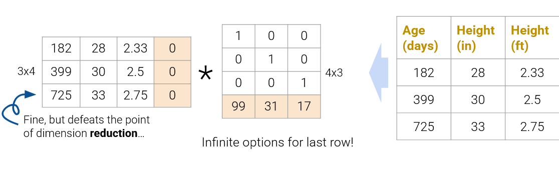
We can even expand the \(3\times3\) matrices to \(3\times4\) and \(4\times3\) (shown below as the factorization on top), but this defeats the point of dimensionality reduction since we’re adding more “useless” dimensions.
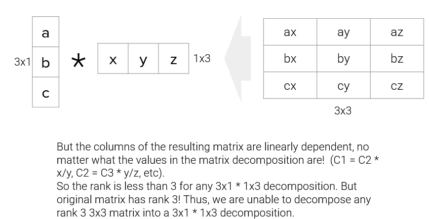
On the flip side, we also can’t reduce the dimension to \(3\times1\) and \(1\times3\) (shown below as the factorization on the bottom); since the rank of the original matrix is greater than 1, this decomposition will not result in the original matrix.
In practice, we often work with datasets containing many features, so we usually want to construct decompositions where the dimensionality is below the rank of the original matrix. While this does not recover the data exactly, we can still provide approximate reconstructions of the matrix.
In the next section, we will discuss a method to automatically and approximately factorize data. This avoids redundant features and makes computation easier because we can train on less data. Since some approximations are better than others, we will also discuss how the method helps us capture a lot of information in a low number of dimensions.
In PCA, our goal is to transform observations from high-dimensional data down to low dimensions (often 2, as most visualizations are 2D) through linear transformations. In other words, we want to find a linear transformation that creates a low-dimension representation that captures as much of the original data’s variability as possible.
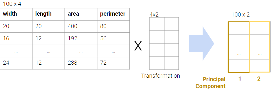
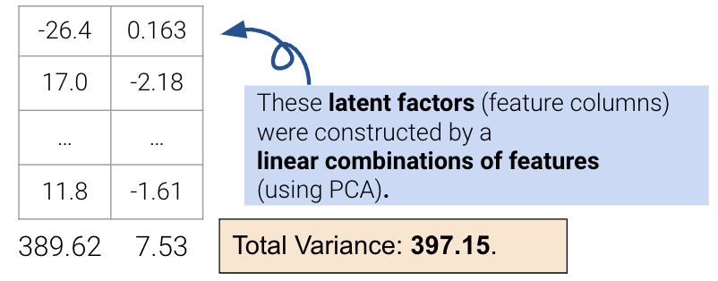
Each column of the transformation matrix is a prinicipal component that describes the basic directions of the data when represented in lower-dimensional space. The columns of the new lower-dimension representation are called the latent factors, and we often work with these to represent and visualize the data. We’ll discuss more about these two terms in a bit.
We often perform PCA during the Exploratory Data Analysis (EDA) stage of our data science lifecycle when we don’t know what model to use. It helps us with:
There are two equivalent ways of framing PCA:
To execute the first approach of variance maximization framing (more common), we can find the variances of each attribute with np.var and then keep the \(k\) attributes with the highest variance. For example, if we are working with data that has the features width, length, area, and perimeter, we can compute the total variance as the sum of the variance in each column. The total variance would be 402.56, and we want to find a representation which captures as much of the original data’s total variance as possible. Here, we choose area and perimeter which captures 389.52 of the original 402.56.

However, this approach limits us to work with attributes individually; it cannot resolve collinearity, and we cannot combine features. The second approach uses PCA to construct latent factors with the most variance in the data (even higher than the first approach) using linear combinations of features.
We’ll describe the procedure for this second approach in the next section.
To perform PCA on a matrix:
The \(k\) principal components capture the most variance of any \(k\)-dimensional reduction of the data matrix. In the example below from Stack Exchange, maximizing variance means spreading out the red dots, and minimizing error (the projections) means making red lines short.
In this section, we will derive PCA keeping the following goal in mind: minimize the reconstruction loss for our matrix factorization model. You are not expected to be able to be able to redo this derivation, but understanding the derivation may help with future assignments.
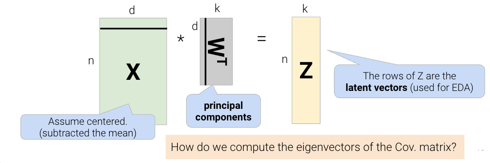
Given a matrix \(X\) with \(n\) rows and \(d\) columns, our goal is to find its best decomposition such that \[X \approx Z W\] Z has \(n\) rows and \(k\) columns; W has \(k\) rows and \(d\) columns. To measure the accuracy of our reconstruction, we define the reconstruction loss below, where \(X_i\) is the row vector of \(X\), and \(Z_i\) is the row vector of \(Z\):
We can then rewrite the norm squared as the matrix product of a row vector and a column vector.
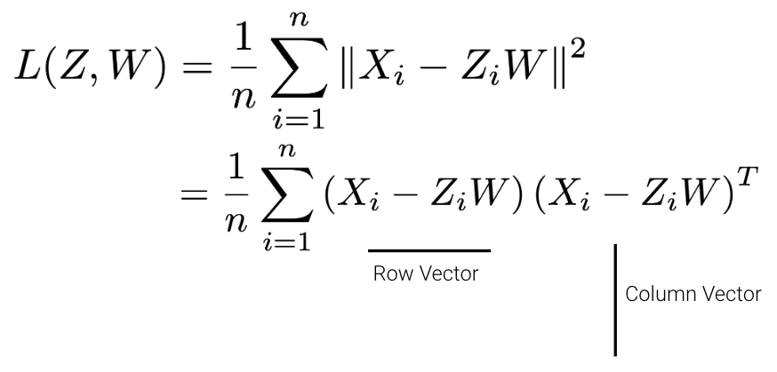
There are many solutions to the above, so let’s constrain our model such that \(W\) is a row-orthonormal matrix (i.e. \(WW^T=I\)) where the rows of \(W\) are our principal components.
In our derivation, let’s first work with the case where \(k=1\). Here Z will be an \(n \times 1\) vector and W will be a \(1 \times d\) vector.
\[\begin{aligned} L(z,w) &= \frac{1}{n}\sum_{i=1}^{n}(X_i - z_{i}w)(X_i - z_{i}w)^T \\ &= \frac{1}{n}\sum_{i=1}^{n}(X_{i}X_{i}^T - 2z_{i}X_{i}w^T + z_{i}^{2}ww^T) \ \ \ \text{(expand the loss)} \\ &= \frac{1}{n}\sum_{i=1}^{n}(-2z_{i}X_{i}w^T + z_{i}^{2}) \ \ \ \text{(First term is constant and }ww^T=1\text{ by orthonormality)} \\ \end{aligned}\]
Now, we can take the derivative with respect to \(z_i\), set the derivative equal to 0, and solve for \(z_i\). \[\begin{aligned} \frac{\partial{L(z,w)}}{\partial{z_i}} &= \frac{1}{n}(-2X_{i}w^T + 2z_{i}) \\ z_i &= X_iw^T \end{aligned}\]
This tells us that we can compute \(z\) by projecting onto \(w\). We can now substitute our solution for \(z_i\) in our loss function:
\[\begin{aligned} L(z,w) &= \frac{1}{n}\sum_{i=1}^{n}(-2z_{i}X_{i}w^T + z_{i}^{2}) \\ L(z=Xw^T,w) &= \frac{1}{n}\sum_{i=1}^{n}(-2X_iw^TX_{i}w^T + (X_iw^T)^{2}) \\ &= \frac{1}{n}\sum_{i=1}^{n}(-X_iw^TX_{i}w^T) \\ &= \frac{1}{n}\sum_{i=1}^{n}(-wX_{i}^TX_{i}w^T) \hspace{1cm} \textcolor{green}{\text{Algebra}}\\ &= -w\frac{1}{n}\sum_{i=1}^{n}(X_i^TX_{i})w^T \\ &= -w\Sigma w^T \hspace{2cm} \textcolor{green}{\text{Definition of Covariance ($\Sigma$)}} \end{aligned}\]
Now, we need to minimize our loss with respect to \(w\). Since we have a negative sign, one way we can do this is by making \(w\) really big. However, we also have the orthonormality constraint \(ww^T=1\). To incorporate this constraint into the equation, we can add a Lagrange multiplier, \(\lambda\). Note that lagrangian multipliers are out of scope for Data 100.
\[ L(w,\lambda) = -w\Sigma w^T + \lambda(ww^T-1) \]
Taking the derivative with respect to \(w\) and setting equal to zero, \[\begin{aligned} \frac{\partial{L(w,\lambda)}}{\partial{w}} &= -2\Sigma w^T + 2\lambda w^T \\ -2\Sigma w^T + 2\lambda w^T &= 0 \\ \Sigma w^T &= \lambda w^T \\ \end{aligned}\]
This result implies that:
This derivation can inductively be used for the next (second) principal component (not shown).
The final takeaway from this derivation is that the principal components are the eigenvectors with the largest eigenvalues of the covariance matrix. These are the directions of the maximum variance of the data. We can construct the latent factors (the Z matrix) by projecting the centered data X onto the principal component vectors: