import numpy as npimport pandas as pdimport matplotlib.pyplot as pltimport seaborn as sns#%matplotlib inlineplt.rcParams['figure.figsize'] = (12, 9)sns.set()sns.set_context('talk')np.set_printoptions(threshold=20, precision=2, suppress=True)pd.set_option('display.max_rows', 30)pd.set_option('display.max_columns', None)pd.set_option('display.precision', 2)# This option stops scientific notation for pandaspd.set_option('display.float_format', '{:.2f}'.format)# Silence some spurious seaborn warningsimport warningswarnings.filterwarnings("ignore", category=FutureWarning)warnings.filterwarnings("ignore", category=UserWarning)
NoteLearning Outcomes
Recognize common file formats
Categorize data by its variable type
Build awareness of issues with data faithfulness and develop targeted solutions
In the past few lectures, we’ve learned that pandas is a toolkit to restructure, modify, and explore a dataset. What we haven’t yet touched on is how to make these data transformation decisions. When we receive a new set of data from the “real world,” how do we know what processing we should do to convert this data into a usable form?
Data cleaning, also called data wrangling, is the process of transforming raw data to facilitate subsequent analysis. It is often used to address issues like:
Unclear structure or formatting
Missing or corrupted values
Unit conversions
…and so on
Exploratory Data Analysis (EDA) is the process of understanding a new dataset. It is an open-ended, informal analysis that involves familiarizing ourselves with the variables present in the data, discovering potential hypotheses, and identifying possible issues with the data. This last point can often motivate further data cleaning to address any problems with the dataset’s format; because of this, EDA and data cleaning are often thought of as an “infinite loop,” with each process driving the other.
In this lecture, we will consider the key properties of data to consider when performing data cleaning and EDA. In doing so, we’ll develop a “checklist” of sorts for you to consider when approaching a new dataset. Throughout this process, we’ll build a deeper understanding of this early (but very important!) stage of the data science lifecycle.
Structure
We often prefer rectangular data for data analysis. Rectangular structures are easy to manipulate and analyze. A key element of data cleaning is about transforming data to be more rectangular.
There are two kinds of rectangular data: tables and matrices. Tables have named columns with different data types and are manipulated using data transformation languages. Matrices contain numeric data of the same type and are manipulated using linear algebra.
File Formats
There are many file types for storing structured data: TSV, JSON, XML, ASCII, SAS, etc. We’ll only cover CSV, TSV, and JSON in lecture, but you’ll likely encounter other formats as you work with different datasets. Reading documentation is your best bet for understanding how to process the multitude of different file types.
CSV
CSVs, which stand for Comma-Separated Values, are a common tabular data format. In the past two pandas lectures, we briefly touched on the idea of file format: the way data is encoded in a file for storage. Specifically, our elections and babynames datasets were stored and loaded as CSVs:
pd.read_csv("data/elections.csv").head(5)
Year
Candidate
Party
Popular vote
Result
%
0
1824
Andrew Jackson
Democratic-Republican
151271
loss
57.21
1
1824
John Quincy Adams
Democratic-Republican
113142
win
42.79
2
1828
Andrew Jackson
Democratic
642806
win
56.20
3
1828
John Quincy Adams
National Republican
500897
loss
43.80
4
1832
Andrew Jackson
Democratic
702735
win
54.57
To better understand the properties of a CSV, let’s take a look at the first few rows of the raw data file to see what it looks like before being loaded into a DataFrame. We’ll use the repr() function to return the raw string with its special characters:
withopen("data/elections.csv", "r") as table: i =0for row in table:print(repr(row)) i +=1if i >3:break
Each row, or record, in the data is delimited by a newline \n. Each column, or field, in the data is delimited by a comma , (hence, comma-separated!).
TSV
Another common file type is TSV (Tab-Separated Values). In a TSV, records are still delimited by a newline \n, while fields are delimited by \t tab character.
Let’s check out the first few rows of the raw TSV file. Again, we’ll use the repr() function so that print shows the special characters.
withopen("data/elections.txt", "r") as table: i =0for row in table:print(repr(row)) i +=1if i >3:break
An issue with CSVs and TSVs comes up whenever there are commas or tabs within the records. How does pandas differentiate between a comma delimiter vs. a comma within the field itself, for example 8,900? To remedy this, check out the quotecharparameter.
JSON
JSON (JavaScript Object Notation) files behave similarly to Python dictionaries. A raw JSON is shown below.
withopen("data/elections.json", "r") as table: i =0for row in table:print(row) i +=1if i >8:break
JSON files can be loaded into pandas using pd.read_json.
pd.read_json('data/elections.json').head(3)
Year
Candidate
Party
Popular vote
Result
%
0
1824
Andrew Jackson
Democratic-Republican
151271
loss
57.21
1
1824
John Quincy Adams
Democratic-Republican
113142
win
42.79
2
1828
Andrew Jackson
Democratic
642806
win
56.20
EDA with JSON: United States Congress Data
The congress.gov API (Application Programming Interface) provides data about the activities and members of the United States Congress (i.e., the House of Representatives and the Senate).
To get a JSON file containing information about the current members of Congress from California, you could use the following API call:
You can instantly sign up for a congress.gov API keyhere. Once you have your key, replace [INSERT_KEY] above with your key, and enter the API call as a URL in your browser. What happens?
Once the JSON from the API call is visible in your browser, you can click File –> Save Page As to save the JSON file to your coputer.
Coarsely, API keys are used to track how much a given user engages with the API. There might be limits to the number of API calls (e.g., congress.gov API limits to 5,000 calls per hour), or a cost for API calls (e.g., using the OpenAI API for programmatically using ChatGPT).
After following these steps, we save this JSON file as data/ca-congress-members.json.
File Contents
Let’s examine this file using Python. We can programmatically view the first couple lines of the file using the same functions we used with CSVs:
congress_file ="data/ca-congress-members.json"# Inspect the first five lines of the filewithopen(congress_file, "r") as f:for i, row inenumerate(f):print(row)if i >=4: break
JSON data closely matches the internal Python object model.
In the following cell, we import the entire JSON datafile into a Python dictionary using the json package.
import json# Import the JSON file into Python as a dictionarywithopen(congress_file, "rb") as f: congress_json = json.load(f)type(congress_json)
dict
The congress_json variable is a dictionary encoding the data in the JSON file.
Below, we access the first element of the members element of the congress_json dictionary.
This first element is also a dictionary (and there are more dictionaries inside of it!)
# Grab the list corresponding to the `members` key in the JSON dictionary, # and then grab the first element of this list.# In a moment, we'll see how we knew to use the key `members`, and that# the resulting object is a list.congress_json['members'][0]
How should we probe a nested dictionary like congress_json?
We can start by identifying the top-level keys of the dictionary:
# Grab the top-level keys of the JSON dictionarycongress_json.keys()
dict_keys(['members', 'pagination', 'request'])
Looks like we have three top-level keys: members, pagination, and request.
You’ll often see a top-level meta key in JSON files. This does not refer to Meta (formerly Facebook). Instead, it typically refers to metadata (data about the data). Metadata are often maintained alongside the data.
Let’s check the type of the members element:
type(congress_json['members'])
list
Looks like a list! What are the first two elements?
pandas has a built in function called pd.read_json for reading in JSON files. In order to read in this JSON file, you might want to try something like the code in the cell below. However, if we tried to run this code, it would error.
#pd.read_json(congress_file)
The code above tries to import the entire JSON file located at congress_file (congress_json), including congress_json['pagination'] and congress_json['request'].
We only want to make a DataFrame out of congress_json['members'].
Instead, let’s try converting the members element of congress_json to a DataFrame by using pd.DataFrame:
# Convert dictionary to DataFramecongress_df = pd.DataFrame(congress_json['members'])congress_df.head()
bioguideId
depiction
district
name
partyName
state
terms
updateDate
url
0
T000491
{'attribution': 'Image courtesy of the Member'...
45.00
Tran, Derek
Democratic
California
{'item': [{'chamber': 'House of Representative...
2025-01-21T18:00:52Z
https://api.congress.gov/v3/member/T000491?for...
1
M001241
{'attribution': 'Image courtesy of the Member'...
47.00
Min, Dave
Democratic
California
{'item': [{'chamber': 'House of Representative...
2025-01-21T18:00:52Z
https://api.congress.gov/v3/member/M001241?for...
2
K000400
{'attribution': 'Image courtesy of the Member'...
37.00
Kamlager-Dove, Sydney
Democratic
California
{'item': [{'chamber': 'House of Representative...
2025-01-21T18:00:52Z
https://api.congress.gov/v3/member/K000400?for...
3
G000598
{'attribution': 'Image courtesy of the Member'...
42.00
Garcia, Robert
Democratic
California
{'item': [{'chamber': 'House of Representative...
2025-01-21T18:00:52Z
https://api.congress.gov/v3/member/G000598?for...
4
K000397
{'attribution': 'Image courtesy of the Member'...
40.00
Kim, Young
Republican
California
{'item': [{'chamber': 'House of Representative...
2025-01-21T18:00:52Z
https://api.congress.gov/v3/member/K000397?for...
We’ve successfully begun to rectangularize our JSON data!
Other Data Formats
So far, we’ve looked at text data that comes in a quite nice format. Although some data cleaning might be necessary, it has still had all of the components of a rectangular dataset. However, not all data comes like this, and there are also different kinds of data we can use. Some examples include:
Image Data: Used for medical diagnosis
Audio Data: Used for speech recognition, sentiment analysis
Video Data: Used for object tracking, facial recognition
Text: Used for LLMs, document review
Even though this may not look tabular at first, all of these formats can be represented in tabular/matrix form! So by learning how to work with tabular data, you are well equipped to deal with other kinds of data as well.
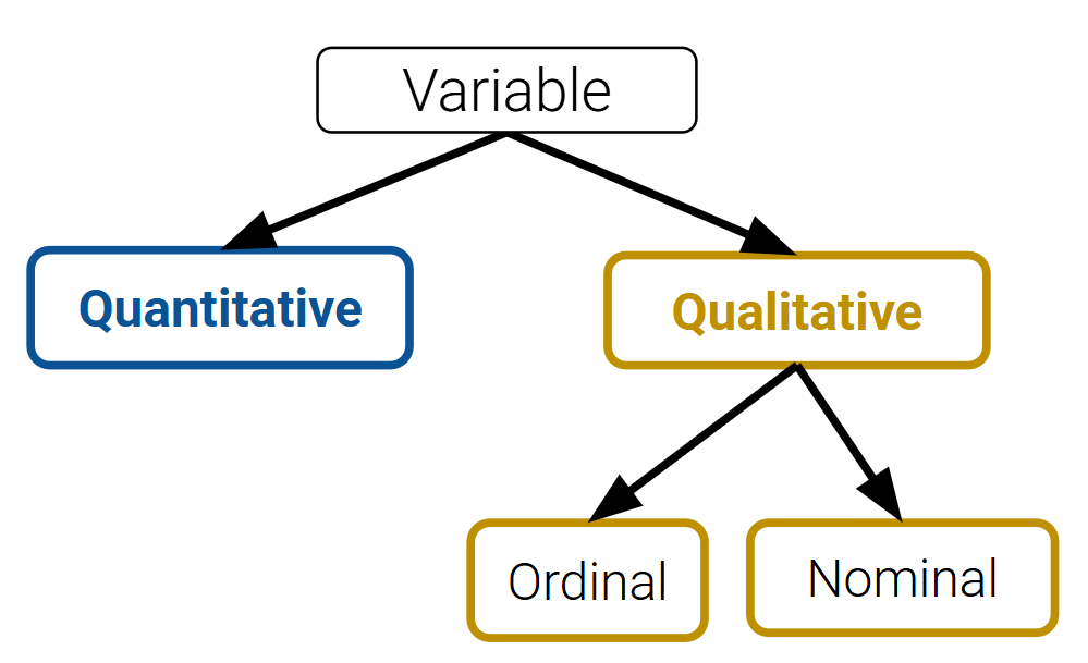
Variable Types
Variables are columns. A variable is a measurement of a particular concept. Variables have two common properties: data type/storage type and variable type/feature type. The data type of a variable indicates how each variable value is stored in memory (integer, floating point, boolean, etc.) and affects which pandas functions are used. The variable type is a conceptualized measurement of information (and therefore indicates what values a variable can take on). Variable type is identified through expert knowledge, exploring the data itself, or consulting the data codebook. The variable type affects how one visualizes and inteprets the data. In this class, “variable types” are conceptual.
After loading data into a file, it’s a good idea to take the time to understand what pieces of information are encoded in the dataset. In particular, we want to identify what variable types are present in our data. Broadly speaking, we can categorize variables into one of two overarching types.
Quantitative variables describe some numeric quantity or amount. Some examples include weights, GPA, CO2 concentrations, someone’s age, or the number of siblings they have.
Qualitative variables, also known as categorical variables, describe data that isn’t measuring some quantity or amount. The sub-categories of categorical data are:
Ordinal qualitative variables: categories with ordered levels. Specifically, ordinal variables are those where the difference between levels has no consistent, quantifiable meaning. Some examples include levels of education (high school, undergrad, grad, etc.), income bracket (low, medium, high), or Yelp rating.
Nominal qualitative variables: categories with no specific order. For example, someone’s political affiliation or Cal ID number.
Note that many variables don’t sit neatly in just one of these categories. Qualitative variables could have numeric levels, and conversely, quantitative variables could be stored as strings.
Granularity and Temporality
After understanding the structure of the dataset, the next task is to determine what exactly the data represents. We’ll do so by considering the data’s granularity and temporality.
Granularity
The granularity of a dataset is what a single row represents. You can also think of it as the level of detail included in the data. To determine the data’s granularity, ask: what does each row in the dataset represent? Fine-grained data contains a high level of detail, with a single row representing a small individual unit. For example, each record may represent one person. Coarse-grained data is encoded such that a single row represents a large individual unit – for example, each record may represent a group of people.
Temporality
The temporality of a dataset describes the periodicity over which the data was collected as well as when the data was most recently collected or updated.
Time and date fields of a dataset could represent a few things:
when the “event” happened
when the data was collected, or when it was entered into the system
when the data was copied into the database
To fully understand the temporality of the data, it also may be necessary to standardize time zones or inspect recurring time-based trends in the data (do patterns recur in 24-hour periods? Over the course of a month? Seasonally?). The convention for standardizing time is the Coordinated Universal Time (UTC), an international time standard measured at 0 degrees latitude that stays consistent throughout the year (no daylight savings). We can represent Berkeley’s time zone, Pacific Standard Time (PST), as UTC-7 (with daylight savings).
Temporality with pandas’ dt accessors
Let’s briefly look at how we can use pandas’ dt accessors to work with dates/times in a dataset using the dataset you’ll see in Lab 3: the Berkeley PD Calls for Service dataset.
Looks like there are three columns with dates/times: EVENTDT, EVENTTM, and InDbDate.
Most likely, EVENTDT stands for the date when the event took place, EVENTTM stands for the time of day the event took place (in 24-hr format), and InDbDate is the date this call is recorded onto the database.
If we check the data type of these columns, we will see they are stored as strings. We can convert them to datetime objects using pandas to_datetime function.
Check the mimimum values to see if there are any suspicious-looking, 70s dates:
calls.sort_values("EVENTDT").head()
CASENO
OFFENSE
EVENTDT
EVENTTM
CVLEGEND
CVDOW
InDbDate
Block_Location
BLKADDR
City
State
2513
20057398
BURGLARY COMMERCIAL
2020-12-17
16:05
BURGLARY - COMMERCIAL
4
06/15/2021 12:00:00 AM
600 BLOCK GILMAN ST\nBerkeley, CA\n(37.878405,...
600 BLOCK GILMAN ST
Berkeley
CA
624
20057207
ASSAULT/BATTERY MISD.
2020-12-17
16:50
ASSAULT
4
06/15/2021 12:00:00 AM
2100 BLOCK SHATTUCK AVE\nBerkeley, CA\n(37.871...
2100 BLOCK SHATTUCK AVE
Berkeley
CA
154
20092214
THEFT FROM AUTO
2020-12-17
18:30
LARCENY - FROM VEHICLE
4
06/15/2021 12:00:00 AM
800 BLOCK SHATTUCK AVE\nBerkeley, CA\n(37.8918...
800 BLOCK SHATTUCK AVE
Berkeley
CA
659
20057324
THEFT MISD. (UNDER $950)
2020-12-17
15:44
LARCENY
4
06/15/2021 12:00:00 AM
1800 BLOCK 4TH ST\nBerkeley, CA\n(37.869888, -...
1800 BLOCK 4TH ST
Berkeley
CA
993
20057573
BURGLARY RESIDENTIAL
2020-12-17
22:15
BURGLARY - RESIDENTIAL
4
06/15/2021 12:00:00 AM
1700 BLOCK STUART ST\nBerkeley, CA\n(37.857495...
1700 BLOCK STUART ST
Berkeley
CA
Doesn’t look like it! We are good!
We can also do many things with the dt accessor like switching time zones and converting time back to UNIX/POSIX time. Check out the documentation on .dtaccessor and time series/date functionality.
Faithfulness
At this stage in our data cleaning and EDA workflow, we’ve achieved quite a lot: we’ve identified how our data is structured, come to terms with what information it encodes, and gained insight as to how it was generated. Throughout this process, we should always recall the original intent of our work in Data Science – to use data to better understand and model the real world. To achieve this goal, we need to ensure that the data we use is faithful to reality; that is, that our data accurately captures the “real world.”
Data used in research or industry is often “messy” – there may be errors or inaccuracies that impact the faithfulness of the dataset. Signs that data may not be faithful include:
Unrealistic or “incorrect” values, such as negative counts, locations that don’t exist, or dates set in the future
Violations of obvious dependencies, like an age that does not match a birthday
Clear signs that data was entered by hand, which can lead to spelling errors or fields that are incorrectly shifted
Signs of data falsification, such as fake email addresses or repeated use of the same names
Duplicated records or fields containing the same information
Truncated data, e.g. Microsoft Excel would limit the number of rows to 655536 and the number of columns to 255
We often solve some of these more common issues in the following ways:
Spelling errors: apply corrections or drop records that aren’t in a dictionary
Time zone inconsistencies: convert to a common time zone (e.g. UTC)
Duplicated records or fields: identify and eliminate duplicates (using primary keys)
Unspecified or inconsistent units: infer the units and check that values are in reasonable ranges in the data
Missing Values
Another common issue encountered with real-world datasets is that of missing data. One strategy to resolve this is to simply drop any records with missing values from the dataset. This does, however, introduce the risk of inducing biases – it is possible that the missing or corrupt records may be systemically related to some feature of interest in the data. Another solution is to keep the data as NaN values.
A third method to address missing data is to perform imputation: infer the missing values using other data available in the dataset. There is a wide variety of imputation techniques that can be implemented; some of the most common are listed below.
Average imputation: replace missing values with the average value for that field
Hot deck imputation: replace missing values with some random value
Regression imputation: develop a model to predict missing values and replace with the predicted value from the model.
Multiple imputation: replace missing values with multiple random values
Regardless of the strategy used to deal with missing data, we should think carefully about why particular records or fields may be missing – this can help inform whether or not the absence of these values is significant or meaningful.
EDA Demo 1: Tuberculosis in the United States
Now, let’s walk through the data-cleaning and EDA workflow to see what can we learn about the presence of Tuberculosis in the United States!
We will examine the data included in the original CDC article published in 2021.
CSVs and Field Names
Suppose Table 1 was saved as a CSV file located in data/cdc_tuberculosis.csv.
We can then explore the CSV (which is a text file, and does not contain binary-encoded data) in many ways: 1. Using a text editor like emacs, vim, VSCode, etc. 2. Opening the CSV directly in DataHub (read-only), Excel, Google Sheets, etc. 3. The Python file object 4. pandas, using pd.read_csv()
To try out options 1 and 2, you can view or download the Tuberculosis from the lecture demo notebook under the data folder in the left hand menu. Notice how the CSV file is a type of rectangular data (i.e., tabular data) stored as comma-separated values.
Next, let’s try out option 3 using the Python file object. We’ll look at the first four lines:
Code
withopen("data/cdc_tuberculosis.csv", "r") as f: i =0for row in f:print(row) i +=1if i >3:break
,No. of TB cases,,

U.S. jurisdiction,2019,2020,2021

Total,"8,900","7,173","7,860"

Alabama,87,72,92
Whoa, why are there blank lines interspaced between the lines of the CSV?
You may recall that all line breaks in text files are encoded as the special newline character \n. Python’s print() prints each string (including the newline), and an additional newline on top of that.
If you’re curious, we can use the repr() function to return the raw string with all special characters:
Code
withopen("data/cdc_tuberculosis.csv", "r") as f: i =0for row in f:print(repr(row)) # print raw strings i +=1if i >3:break
',No. of TB cases,,\n'
'U.S. jurisdiction,2019,2020,2021\n'
'Total,"8,900","7,173","7,860"\n'
'Alabama,87,72,92\n'
Finally, let’s try option 4 and use the tried-and-true Data 100 approach: pandas.
You may notice some strange things about this table: what’s up with the “Unnamed” column names and the first row?
Congratulations — you’re ready to wrangle your data! Because of how things are stored, we’ll need to clean the data a bit to name our columns better.
A reasonable first step is to identify the row with the right header. The pd.read_csv() function (documentation) has the convenient header parameter that we can set to use the elements in row 1 as the appropriate columns:
You might already be wondering: what’s up with that first record?
Row 0 is what we call a rollup record, or summary record. It’s often useful when displaying tables to humans. The granularity of record 0 (Totals) vs the rest of the records (States) is different.
Okay, EDA step two. How was the rollup record aggregated?
Let’s check if Total TB cases is the sum of all state TB cases. If we sum over all rows, we should get 2x the total cases in each of our TB cases by year (why do you think this is?).
Since there are commas in the values for TB cases, the numbers are read as the object datatype, or storage type (close to the Python string datatype), so pandas is concatenating strings instead of adding integers (recall that Python can “sum”, or concatenate, strings together: "data" + "100" evaluates to "data100").
Fortunately read_csv also has a thousands parameter (documentation):
Let’s just look at the records with state-level granularity:
Code
state_tb_df = tb_df[1:]state_tb_df.head(5)
U.S. jurisdiction
2019
2020
2021
1
Alabama
87
72
92
2
Alaska
58
58
58
3
Arizona
183
136
129
4
Arkansas
64
59
69
5
California
2111
1706
1750
Gather Census Data
U.S. Census population estimates source (2019), source (2020-2024).
Running the below cells cleans the data. There are a few new methods here:
df.convert_dtypes() (documentation) conveniently converts all float dtypes into ints and is out of scope for the class.
df.drop_na() (documentation) will be explained in more detail next time.
Code
# 2010s census datacensus_2010s_df = pd.read_csv("data/nst-est2019-01.csv", header=3, thousands=",")census_2010s_df = ( census_2010s_df .rename(columns={"Unnamed: 0": "Geographic Area"}) .drop(columns=["Census", "Estimates Base"]) .convert_dtypes() # "smart" converting of columns to int, use at your own risk .dropna() # we'll introduce this very soon)census_2010s_df['Geographic Area'] = census_2010s_df['Geographic Area'].str.strip('.')# with pd.option_context('display.min_rows', 30): # shows more rows# display(census_2010s_df)census_2010s_df.head(5)
Geographic Area
2010
2011
2012
2013
2014
2015
2016
2017
2018
2019
0
United States
309321666
311556874
313830990
315993715
318301008
320635163
322941311
324985539
326687501
328239523
1
Northeast
55380134
55604223
55775216
55901806
56006011
56034684
56042330
56059240
56046620
55982803
2
Midwest
66974416
67157800
67336743
67560379
67745167
67860583
67987540
68126781
68236628
68329004
3
South
114866680
116006522
117241208
118364400
119624037
120997341
122351760
123542189
124569433
125580448
4
West
72100436
72788329
73477823
74167130
74925793
75742555
76559681
77257329
77834820
78347268
Occasionally, you will want to modify code that you have imported. To reimport those modifications you can either use python’s importlib library:
from importlib importreloadreload(utils)
or use iPython magic which will intelligently import code when files change:
%load_ext autoreload%autoreload 2
Code
# census 2020s datacensus_2020s_df = pd.read_csv("data/NST-EST2024-POP.csv", header=3, thousands=",")census_2020s_df = ( census_2020s_df .drop(columns=["Unnamed: 1"]) .rename(columns={"Unnamed: 0": "Geographic Area"}) .loc[:, "Geographic Area":"2024"] # ignore all the blank extra columns .convert_dtypes() # "smart" converting of columns, use at your own risk .dropna() # we'll introduce this next ti)census_2020s_df['Geographic Area'] = census_2020s_df['Geographic Area'].str.strip('.')census_2020s_df.head(5)
Geographic Area
2020
2021
2022
2023
2024
0
United States
331577720
332099760
334017321
336806231
340110988
1
Northeast
57431458
57252533
57159597
57398303
57832935
2
Midwest
68984258
68872831
68903297
69186401
69596584
3
South
126476549
127368010
129037849
130893358
132665693
4
West
78685455
78606386
78916578
79328169
80015776
Joining Data (Merging DataFrames)
Time to merge! Here we use the DataFrame method df1.merge(right=df2, ...) on DataFramedf1 (documentation). Contrast this with the function pd.merge(left=df1, right=df2, ...) (documentation). Feel free to use either.
# merge TB DataFrame with two US census DataFramestb_census_df = ( tb_df .merge(right=census_2010s_df, left_on="U.S. jurisdiction", right_on="Geographic Area") .merge(right=census_2020s_df, left_on="U.S. jurisdiction", right_on="Geographic Area"))tb_census_df.head(5)
U.S. jurisdiction
2019_x
2020_x
2021_x
Geographic Area_x
2010
2011
2012
2013
2014
2015
2016
2017
2018
2019_y
Geographic Area_y
2020_y
2021_y
2022
2023
2024
0
Alabama
87
72
92
Alabama
4785437
4799069
4815588
4830081
4841799
4852347
4863525
4874486
4887681
4903185
Alabama
5033094
5049196
5076181
5117673
5157699
1
Alaska
58
58
58
Alaska
713910
722128
730443
737068
736283
737498
741456
739700
735139
731545
Alaska
733017
734420
734442
736510
740133
2
Arizona
183
136
129
Arizona
6407172
6472643
6554978
6632764
6730413
6829676
6941072
7044008
7158024
7278717
Arizona
7187135
7274078
7377566
7473027
7582384
3
Arkansas
64
59
69
Arkansas
2921964
2940667
2952164
2959400
2967392
2978048
2989918
3001345
3009733
3017804
Arkansas
3014546
3026870
3047704
3069463
3088354
4
California
2111
1706
1750
California
37319502
37638369
37948800
38260787
38596972
38918045
39167117
39358497
39461588
39512223
California
39521958
39142565
39142414
39198693
39431263
We’re only interested in the population for the years 2019, 2020, and 2021, so let’s select just those columns:
Notice that the columns containing the join keys have all been retained, and all contain the same values.
Furthermore, notice that the duplicated columns are appended with _x and _y to keep the column names unique.
In the TB case count data, column 2019 represents the number of TB cases in 2019, but in the Census data, column 2019 represents the U.S. population.
We can use the suffixes argument to modify the _x and _y defaults to our liking (documentation).
# Specify the suffixes to use for duplicated column namestb_df.merge(right=census_2019_df, left_on="U.S. jurisdiction", right_on="Geographic Area", suffixes=('_cases', '_population')).head()
U.S. jurisdiction
2019_cases
2020
2021
Geographic Area
2019_population
0
Alabama
87
72
92
Alabama
4903185
1
Alaska
58
58
58
Alaska
731545
2
Arizona
183
136
129
Arizona
7278717
3
Arkansas
64
59
69
Arkansas
3017804
4
California
2111
1706
1750
California
39512223
Notice the _x and _y have changed to _cases and _population, just like we specified.
Putting it all together, and dropping the duplicated Geographic Area columns:
# Redux: merge TB dataframe with two US census dataframestb_census_df = ( tb_df .merge(right=census_2019_df, left_on="U.S. jurisdiction", right_on="Geographic Area", suffixes=('_cases', '_population')) .drop(columns="Geographic Area") .merge(right=census_2020_2021_df, left_on="U.S. jurisdiction", right_on="Geographic Area", suffixes=('_cases', '_population')) .drop(columns="Geographic Area"))tb_census_df.tail(2)
U.S. jurisdiction
2019_cases
2020_cases
2021_cases
2019_population
2020_population
2021_population
49
Wisconsin
51
35
66
5822434
5897375
5881608
50
Wyoming
1
0
3
578759
577681
579636
Reproducing Data: Compute Incidence
Let’s see if we can reproduce the original CDC numbers from our augmented dataset of TB case counts and state populations.
Recall that the nationwide TB incidence was 2.7 in 2019, 2.2 in 2020, and 2.4 in 2021.
Along the way, we’ll also compute state-level incidence.
From the CDC report: TB incidence is computed as “Cases per 100,000 persons using mid-year population estimates from the U.S. Census Bureau.”
Let’s start with a simpler question: What is the per person incidence?
In other words, what is the probability that a randomly selected person in the population had TB within a given year?
\[\text{TB incidence per person} = \frac{\text{\# TB cases in population}}{\text{Total population size}}\]
Let’s calculate per person incidence for 2019:
# Calculate per person incidence for 2019tb_census_df["per person incidence 2019"] = ( tb_census_df["2019_cases"]/tb_census_df["2019_population"])tb_census_df
U.S. jurisdiction
2019_cases
2020_cases
2021_cases
2019_population
2020_population
2021_population
per person incidence 2019
0
Alabama
87
72
92
4903185
5033094
5049196
0.00
1
Alaska
58
58
58
731545
733017
734420
0.00
2
Arizona
183
136
129
7278717
7187135
7274078
0.00
3
Arkansas
64
59
69
3017804
3014546
3026870
0.00
4
California
2111
1706
1750
39512223
39521958
39142565
0.00
...
...
...
...
...
...
...
...
...
46
Virginia
191
169
161
8535519
8637615
8658910
0.00
47
Washington
221
163
199
7614893
7727209
7743760
0.00
48
West Virginia
9
13
7
1792147
1791646
1785618
0.00
49
Wisconsin
51
35
66
5822434
5897375
5881608
0.00
50
Wyoming
1
0
3
578759
577681
579636
0.00
51 rows × 8 columns
TB is really rare in the United States, so per person TB incidence is really low, as expected.
But, if we were to consider 100,000 people, the probability of seeing a TB case is higher.
In fact, it would be 100,000 times higher!
\[\text{TB incidence per 100,000} = \text{100,000} * \text{TB incidence per person}\]
# To help read bigger numbers in Python, you can use _ to separate thousands,# akin to using commas. 100_000 is the same as writing 100000, but more readable.tb_census_df["per 100k incidence 2019"] = (100_000* tb_census_df["per person incidence 2019"] )tb_census_df
U.S. jurisdiction
2019_cases
2020_cases
2021_cases
2019_population
2020_population
2021_population
per person incidence 2019
per 100k incidence 2019
0
Alabama
87
72
92
4903185
5033094
5049196
0.00
1.77
1
Alaska
58
58
58
731545
733017
734420
0.00
7.93
2
Arizona
183
136
129
7278717
7187135
7274078
0.00
2.51
3
Arkansas
64
59
69
3017804
3014546
3026870
0.00
2.12
4
California
2111
1706
1750
39512223
39521958
39142565
0.00
5.34
...
...
...
...
...
...
...
...
...
...
46
Virginia
191
169
161
8535519
8637615
8658910
0.00
2.24
47
Washington
221
163
199
7614893
7727209
7743760
0.00
2.90
48
West Virginia
9
13
7
1792147
1791646
1785618
0.00
0.50
49
Wisconsin
51
35
66
5822434
5897375
5881608
0.00
0.88
50
Wyoming
1
0
3
578759
577681
579636
0.00
0.17
51 rows × 9 columns
Now we’re seeing more human-readable values.
For example, there 5.3 tuberculosis cases for every 100,000 California residents in 2019.
To wrap up this exercise, let’s calculate the nationwide incidence of TB in 2019.
# Recall that the CDC reported an incidence of 2.7 per 100,000 in 2019.tot_tb_cases_50_states = tb_census_df["2019_cases"].sum()tot_pop_50_states = tb_census_df["2019_population"].sum()tb_per_100k_50_states =100_000* tot_tb_cases_50_states / tot_pop_50_statestb_per_100k_50_states
2.7114346007625656
We can use a for loop to compute the incidence for 2019, 2020, and 2021.
You’ll notice that we get the same numbers reported by the CDC!
# f strings (f"...") are a handy way to pass in variables to strings.for year in [2019, 2020, 2021]: tot_tb_cases_50_states = tb_census_df[f"{year}_cases"].sum() tot_pop_50_states = tb_census_df[f"{year}_population"].sum() tb_per_100k_50_states =100_000* tot_tb_cases_50_states / tot_pop_50_statesprint(tb_per_100k_50_states)
The values are separated by white space, possibly tabs.
The data line up down the rows. For example, the month appears in 7th to 8th position of each line.
The 71st and 72nd lines in the file contain column headings split over two lines.
We can use read_csv to read the data into a pandasDataFrame, and we provide several arguments to specify that the separators are white space, there is no header (we will set our own column names), and to skip the first 72 rows of the file.
co2 = pd.read_csv( co2_file, header =None, skiprows =72, sep =r'\s+'#delimiter for continuous whitespace (stay tuned for regex next lecture)))co2.head()
0
1
2
3
4
5
6
0
1958
3
1958.21
315.71
315.71
314.62
-1
1
1958
4
1958.29
317.45
317.45
315.29
-1
2
1958
5
1958.38
317.50
317.50
314.71
-1
3
1958
6
1958.46
-99.99
317.10
314.85
-1
4
1958
7
1958.54
315.86
315.86
314.98
-1
Congratulations! You’ve wrangled the data!
…But our columns aren’t named. We need to do more EDA.
Exploring Variable Feature Types
The NOAA webpage might have some useful tidbits (in this case it doesn’t).
Using this information, we’ll rerun pd.read_csv, but this time with some custom column names.
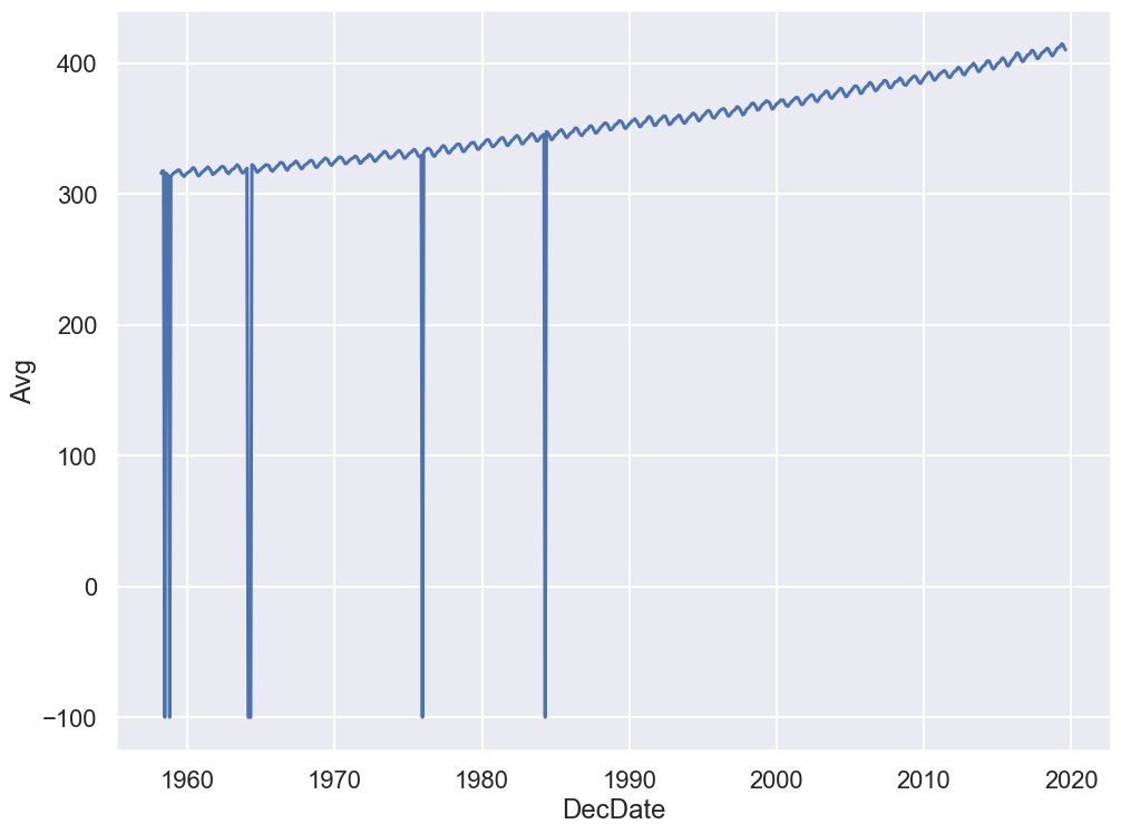
Scientific studies tend to have very clean data, right…? Let’s jump right in and make a time series plot of CO2 monthly averages.
Code
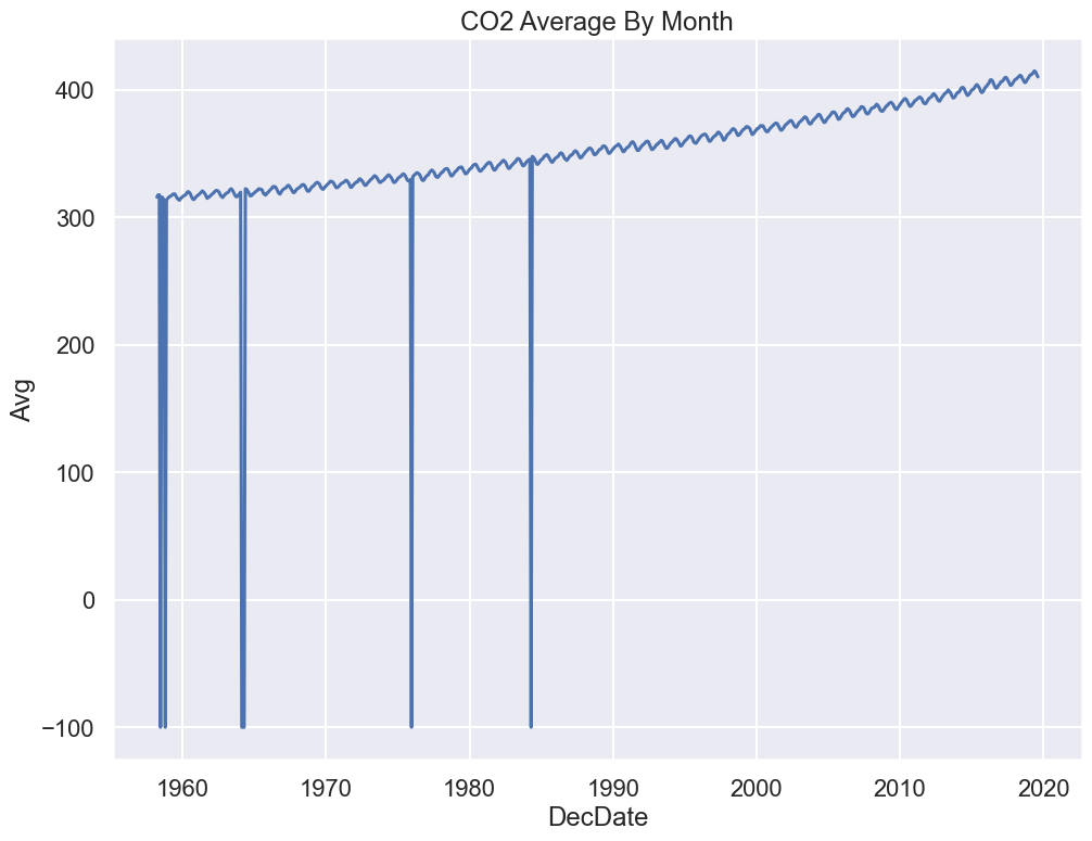
sns.lineplot(x='DecDate', y='Avg', data=co2);
The code above uses the seaborn plotting library (abbreviated sns). We will cover this in the Visualization lecture, but now you don’t need to worry about how it works!
Yikes! Plotting the data uncovered a problem. The sharp vertical lines suggest that we have some missing values. What happened here?
co2.head()
Yr
Mo
DecDate
Avg
Int
Trend
Days
0
1958
3
1958.21
315.71
315.71
314.62
-1
1
1958
4
1958.29
317.45
317.45
315.29
-1
2
1958
5
1958.38
317.50
317.50
314.71
-1
3
1958
6
1958.46
-99.99
317.10
314.85
-1
4
1958
7
1958.54
315.86
315.86
314.98
-1
co2.tail()
Yr
Mo
DecDate
Avg
Int
Trend
Days
733
2019
4
2019.29
413.32
413.32
410.49
26
734
2019
5
2019.38
414.66
414.66
411.20
28
735
2019
6
2019.46
413.92
413.92
411.58
27
736
2019
7
2019.54
411.77
411.77
411.43
23
737
2019
8
2019.62
409.95
409.95
411.84
29
Some data have unusual values like -1 and -99.99.
Let’s check the description at the top of the file again.
-1 signifies a missing value for the number of days Days the equipment was in operation that month.
-99.99 denotes a missing monthly average Avg
How can we fix this? First, let’s explore other aspects of our data. Understanding our data will help us decide what to do with the missing values.
Sanity Checks: Reasoning about the data
First, we consider the shape of the data. How many rows should we have?
If chronological order, we should have one record per month.
Data from March 1958 to August 2019.
We should have $ 12 (2019-1957) - 2 - 4 = 738 $ records.
co2.shape
(738, 7)
Nice!! The number of rows (i.e. records) match our expectations.
Let’s now check the quality of each feature.
Understanding Missing Value 1: Days
Days is a time field, so let’s analyze other time fields to see if there is an explanation for missing values of days of operation.
Let’s start with months, Mo.
Are we missing any records? The number of months should have 62 or 61 instances (March 1957-August 2019).
As expected Jan, Feb, Sep, Oct, Nov, and Dec have 61 occurrences and the rest 62.
Next let’s explore daysDays itself, which is the number of days that the measurement equipment worked.
Code
sns.displot(co2['Days']);plt.title("Distribution of days feature");# suppresses unneeded plotting output
In terms of data quality, a handful of months have averages based on measurements taken on fewer than half the days. In addition, there are nearly 200 missing values–that’s about 27% of the data!
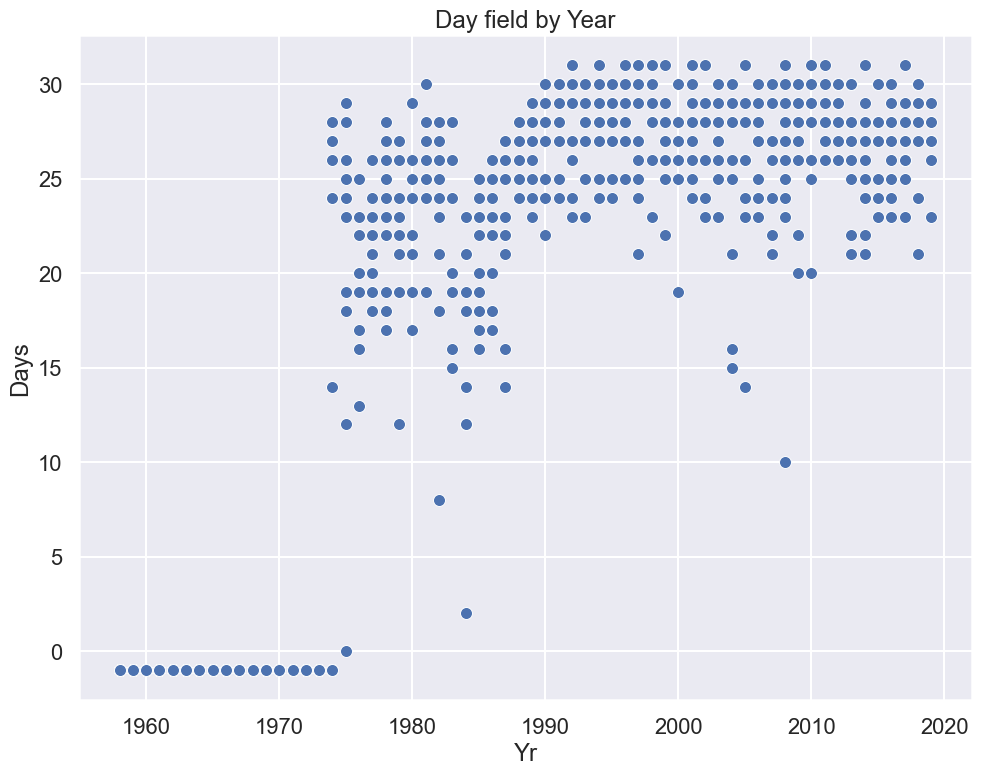
Finally, let’s check the last time feature, yearYr.
Let’s check to see if there is any connection between missing-ness and the year of the recording.
Code
sns.scatterplot(x="Yr", y="Days", data=co2);plt.title("Day field by Year");# the ; suppresses output
Observations:
All of the missing data are in the early years of operation.
It appears there may have been problems with equipment in the mid to late 80s.
Potential Next Steps:
Confirm these explanations through documentation about the historical readings.
Maybe drop the earliest recordings? However, we would want to delay such action until after we have examined the time trends and assess whether there are any potential problems.
Understanding Missing Value 2: Avg
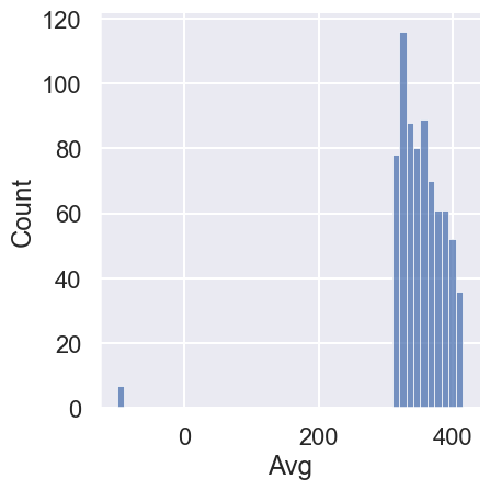
Next, let’s return to the -99.99 values in Avg to analyze the overall quality of the CO2 measurements. We’ll plot a histogram of the average CO2 measurements
Code
# Histograms of average CO2 measurementssns.displot(co2['Avg']);
The non-missing values are in the 300-400 range (a regular range of CO2 levels).
We also see that there are only a few missing Avg values (<1% of values). Let’s examine all of them:
co2[co2["Avg"] <0]
Yr
Mo
DecDate
Avg
Int
Trend
Days
3
1958
6
1958.46
-99.99
317.10
314.85
-1
7
1958
10
1958.79
-99.99
312.66
315.61
-1
71
1964
2
1964.12
-99.99
320.07
319.61
-1
72
1964
3
1964.21
-99.99
320.73
319.55
-1
73
1964
4
1964.29
-99.99
321.77
319.48
-1
213
1975
12
1975.96
-99.99
330.59
331.60
0
313
1984
4
1984.29
-99.99
346.84
344.27
2
There doesn’t seem to be a pattern to these values, other than that most records also were missing Days data.
Drop, NaN, or Impute Missing Avg Data?
How should we address the invalid Avg data?
Drop records
Set to NaN
Impute using some strategy
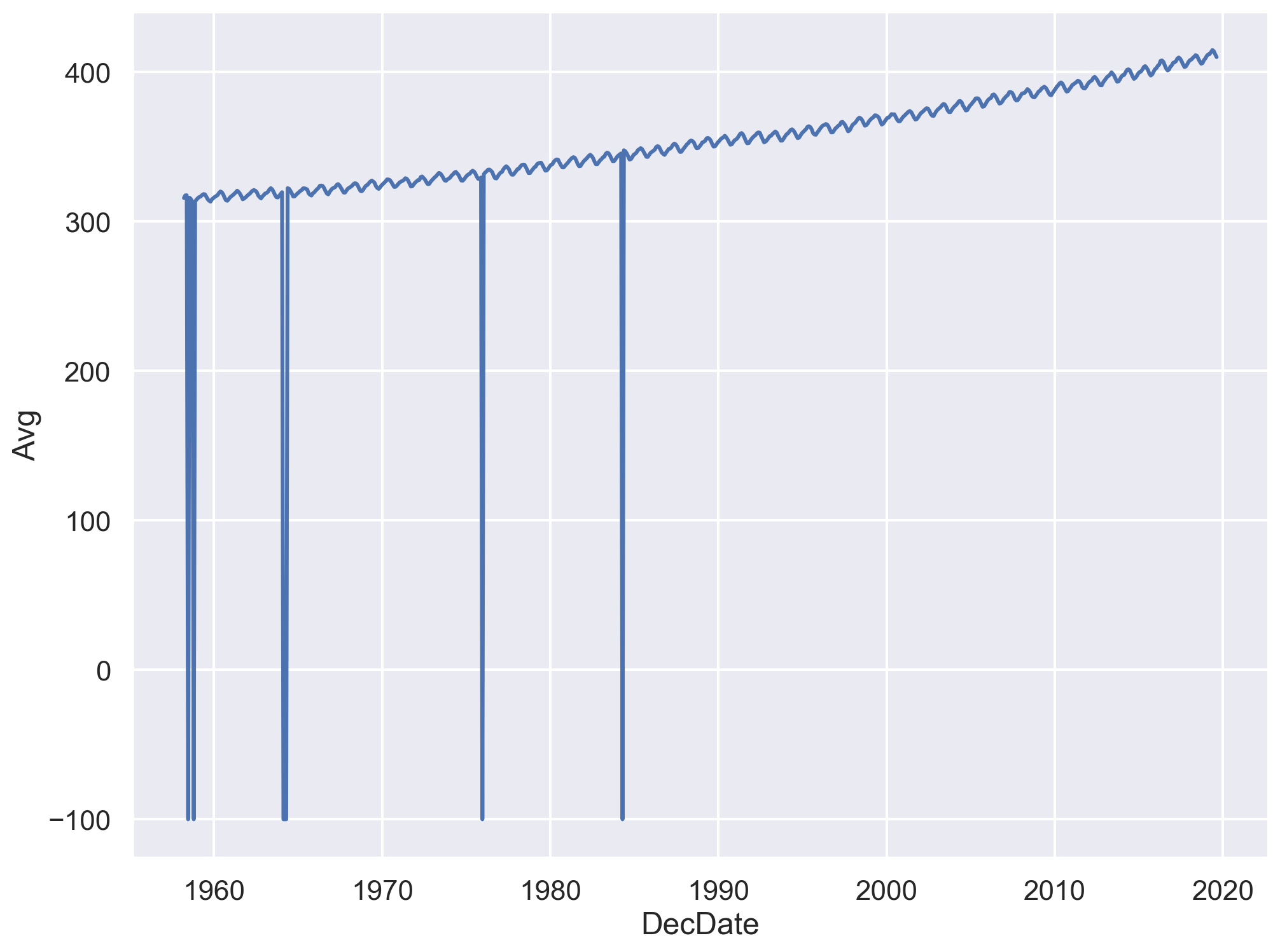
Remember we want to fix the following plot:
Code
sns.lineplot(x='DecDate', y='Avg', data=co2)plt.title("CO2 Average By Month");
Since we are plotting Avg vs DecDate, we should just focus on dealing with missing values for Avg.
Let’s consider a few options: 1. Drop those records 2. Replace -99.99 with NaN 3. Substitute it with a likely value for the average CO2?
What do you think are the pros and cons of each possible action?
Let’s examine each of these three options.
# 1. Drop missing valuesco2_drop = co2[co2['Avg'] >0]co2_drop.head()
Yr
Mo
DecDate
Avg
Int
Trend
Days
0
1958
3
1958.21
315.71
315.71
314.62
-1
1
1958
4
1958.29
317.45
317.45
315.29
-1
2
1958
5
1958.38
317.50
317.50
314.71
-1
4
1958
7
1958.54
315.86
315.86
314.98
-1
5
1958
8
1958.62
314.93
314.93
315.94
-1
# 2. Replace NaN with -99.99co2_NA = co2.replace(-99.99, np.nan)co2_NA.head()
Yr
Mo
DecDate
Avg
Int
Trend
Days
0
1958
3
1958.21
315.71
315.71
314.62
-1
1
1958
4
1958.29
317.45
317.45
315.29
-1
2
1958
5
1958.38
317.50
317.50
314.71
-1
3
1958
6
1958.46
NaN
317.10
314.85
-1
4
1958
7
1958.54
315.86
315.86
314.98
-1
We’ll also use a third version of the data.
First, we note that the dataset already comes with a substitute value for the -99.99.
From the file description:
The interpolated column includes average values from the preceding column (average) and interpolated values where data are missing. Interpolated values are computed in two steps…
The Int feature has values that exactly match those in Avg, except when Avg is -99.99, and then a reasonable estimate is used instead.
So, the third version of our data will use the Int feature instead of Avg.
# 3. Use interpolated column which estimates missing Avg valuesco2_impute = co2.copy()co2_impute['Avg'] = co2['Int']co2_impute.head()
Yr
Mo
DecDate
Avg
Int
Trend
Days
0
1958
3
1958.21
315.71
315.71
314.62
-1
1
1958
4
1958.29
317.45
317.45
315.29
-1
2
1958
5
1958.38
317.50
317.50
314.71
-1
3
1958
6
1958.46
317.10
317.10
314.85
-1
4
1958
7
1958.54
315.86
315.86
314.98
-1
What’s a reasonable estimate?
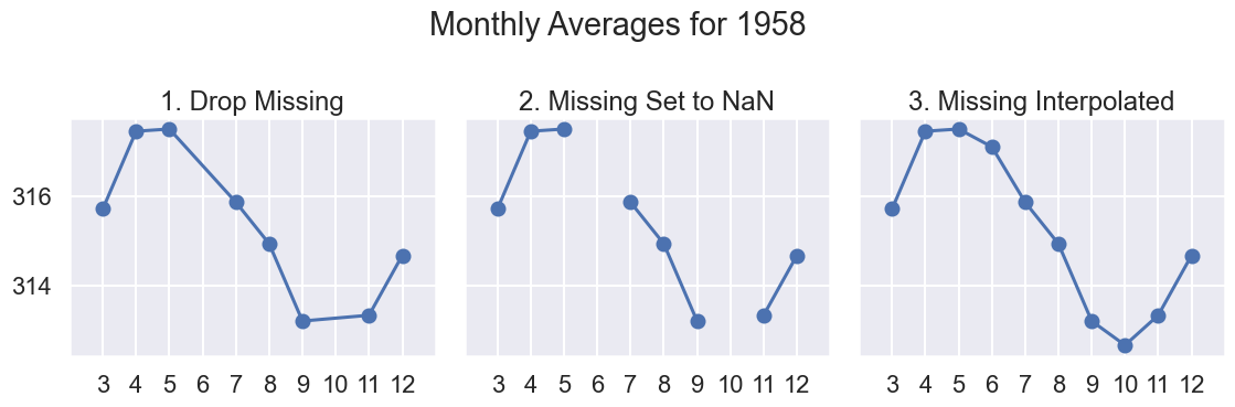
To answer this question, let’s zoom in on a short time period, say the measurements in 1958 (where we know we have two missing values).
Code
# results of plotting data in 1958def line_and_points(data, ax, title):# axssumes single year, hence Mo ax.plot('Mo', 'Avg', data=data) ax.scatter('Mo', 'Avg', data=data) ax.set_xlim(2, 13) ax.set_title(title) ax.set_xticks(np.arange(3, 13))def data_year(data, year):return data[data["Yr"] ==1958]# uses matplotlib subplots# you may see more next week; focus on output for nowfig, axes = plt.subplots(ncols =3, figsize=(12, 4), sharey=True)year =1958line_and_points(data_year(co2_drop, year), axes[0], title="1. Drop Missing")line_and_points(data_year(co2_NA, year), axes[1], title="2. Missing Set to NaN")line_and_points(data_year(co2_impute, year), axes[2], title="3. Missing Interpolated")fig.suptitle(f"Monthly Averages for {year}")plt.tight_layout()
In the big picture since there are only 7 Avg values missing (<1% of 738 months), any of these approaches would work.
However there is some appeal to option C, Imputing:
Shows seasonal trends for CO2
We are plotting all months in our data as a line plot
Let’s replot our original figure with option 3:
Code
sns.lineplot(x='DecDate', y='Avg', data=co2_impute)plt.title("CO2 Average By Month, Imputed");
Looks pretty close to what we see on the NOAA website!
Presenting the Data: A Discussion on Data Granularity
From the description:
Monthly measurements are averages of average day measurements.
The NOAA GML website has datasets for daily/hourly measurements too.
The data you present depends on your research question.
How do CO2 levels vary by season?
You might want to keep average monthly data.
Are CO2 levels rising over the past 50+ years, consistent with global warming predictions?
You might be happier with a coarser granularity of average year data!
Code
co2_year = co2_impute.groupby('Yr').mean()sns.lineplot(x='Yr', y='Avg', data=co2_year)plt.title("CO2 Average By Year");
Indeed, we see a rise by nearly 100 ppm of CO2 since Mauna Loa began recording in 1958.