Construct confidence intervals for hypothesis testing using bootstrapping
Understand the assumptions we make and their impact on our regression inference
Explore ways to overcome issues of multicollinearity
Compare regression correlation and causation
Last time, we introduced the idea of random variables and how they affect the data and model we construct. We also demonstrated the decomposition of model risk from a fitted model and dived into the bias-variance tradeoff.
In this lecture, we will explore regression inference via hypothesis testing, understand how to use bootstrapping under the right assumptions, and consider the environment of understanding causality in theory and in practice.
Review: Bootstrap Resampling
Example: Average Height of UC Berkeley Undegraduates
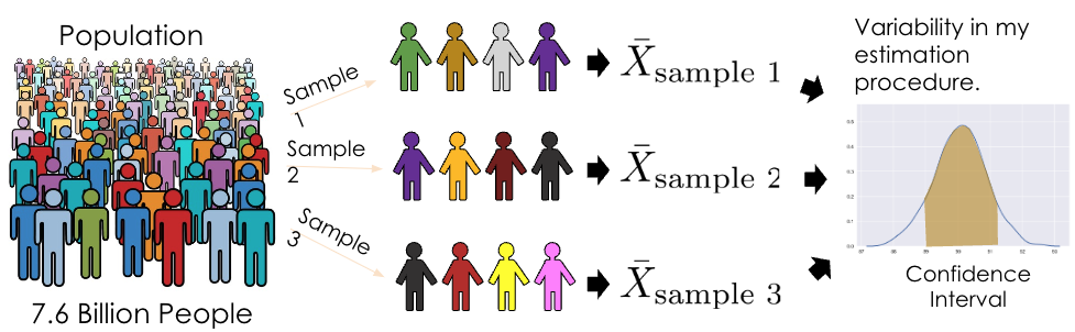
To determine the properties (e.g., variance) of the sampling distribution of an estimator, we’d need access to the population. Ideally, we’d want to consider all possible samples in the population, compute an estimate for each sample, and study the distribution of those estimates.
However, this can be quite expensive and time-consuming. Even more importantly, we don’t have access to the population — we only have one random sample from the population. How can we consider all possible samples if we only have one?
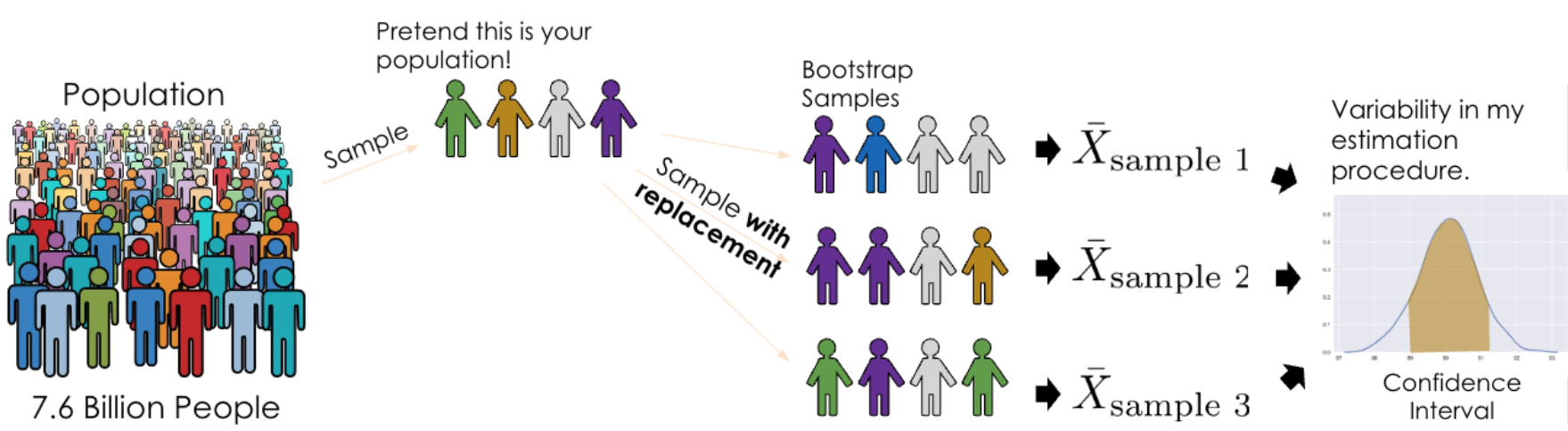
Bootstrapping comes in handy here! With bootstrapping, we treat our random sample as a “population” and resample from it with replacement. Intuitively, a random sample is representative of the population (if it is big enough), so sampling from our sample approximates sampling from the population. When sampling, there are a couple things to keep in mind:
We need to sample the same way we constructed the original sample. Typically, this involves taking a simple random sample with replacement.
New samples must be the same size as the original sample. We need to accurately model the variability of our estimates.
As Professor Grossman noted, we are essentially creating “parallel universes” via bootstrapping the sample.
CautionWhy must we resample with replacement?
Given an original sample of size \(n\), we want a resample that has the same size \(n\) as the original. Sampling without replacement will give us the original sample with shuffled rows. Hence, when we calculate summary statistics like the average, our sample without replacement will always have the same average as the original sample, defeating the purpose of a bootstrap.
Bootstrap resampling is a technique for estimating the sampling distribution of an estimator. Here are the steps of bootstrapping written out:
Assume that your random sample of size \(n\) is representative of the true population.
To mimic a random draw of size \(n\) from the true population, randomly resample \(n\) observations with replacement from your random sample. Call this a “synthetic” random sample.
To compute a synthetic “best guess”, calculate the sample statistic using your synthetic random sample. For example, you could calculate the sample average.
Repeat steps 1 and 2 many times. A common choice is 10,000 times.
The distribution of the 10,000 synthetic “best guesses” provide a sense of uncertainty around your original “best guess”.
From here, we can construct a 95% confidence interval by taking the 2.5% and (100 - 2.5)% percentiles of our bootstrapped thetas.
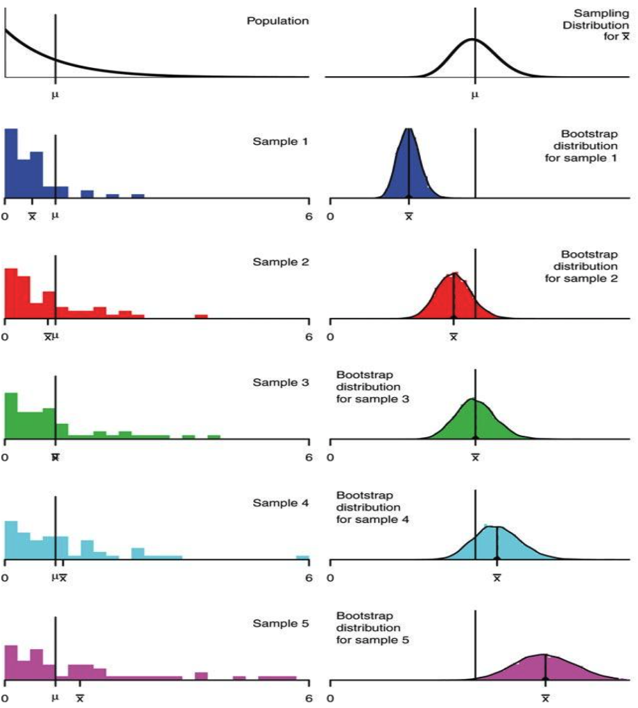
How well does bootstrapping actually represent our population? The bootstrapped sampling distribution of an estimator does not exactly match the sampling distribution of that estimator, but it is often close. Similarly, the variance of the bootstrapped distribution is often close to the true variance of the estimator. The example below displays the results of different bootstraps from a known population using a sample size of \(n=50\).
In the real world, we don’t know the population distribution. The center of the bootstrapped distribution is the estimator applied to our original sample, so we have no way of understanding the estimator’s true expected value; the center and spread of our bootstrap are approximations. The bootstrap does not improve our estimate. The quality of our bootstrapped distribution also depends on the quality of our original sample. If our original sample was not representative of the population (like Sample 5 in the image above), then the bootstrap is next to useless.
NoteBootstrap limitations
In general, bootstrapping works better for large samples, when the population distribution is not heavily skewed (no outliers), and when the estimator is “low variance” (insensitive to extreme values).
Example: Bootstrapping a Regression Coefficient
To get a better idea of how bootstrapping works in practice, let’s walk through a simple example of bootstrapping to estimate the relationship between miles per gallon and the weight of a vehicle. We observe this SLR model: \[
\widehat{\text{mpg}} = \hat{\theta}_0 + \hat{\theta}_1 * \text{weight}
\]
Suppose we collected a sample of 20 cars from a population. For the purposes of this demo, we will assume that the seaborn’s mpg dataset represents the entire population. The following is a visualization of our sample:
Code
import numpy as npimport pandas as pdimport plotly.express as pximport sklearn.linear_model as lmimport seaborn as snsnp.random.seed(42)sample_size =100mpg = sns.load_dataset('mpg')print("Full Data Size:", len(mpg))mpg_sample = mpg.sample(sample_size)print("Sample Size:", len(mpg_sample))px.scatter(mpg_sample, x='weight', y='mpg', trendline='ols', width=800)
Full Data Size: 398
Sample Size: 100
Fitting a linear model, we get an estimate of the slope \(\hat{\theta}_1\):
model = lm.LinearRegression().fit(mpg_sample[['weight']], mpg_sample['mpg'])model.coef_[0]
-0.007305965155512159
Bootstrap Implementation
We can use bootstrapping to estimate the distribution of that coefficient. Here we construct a bootstrap function that takes an estimator function and uses that function to construct many bootstrap estimates of the slope.
def estimator(sample):""" Fits an SLR to `sample` regressing mpg on weight, and returns the slope of the fitted line """ model = lm.LinearRegression().fit(sample[['weight']], sample['mpg'])return model.coef_[0]
The code below uses df.sample(documentation) to generate a bootstrap sample that is the same size as the original sample.
def bootstrap(sample, statistic, num_repetitions):""" Returns the statistic computed on a num_repetitions bootstrap samples from sample. """ stats = []for i in np.arange(num_repetitions):# Step 1: Resample with replacement from our original sample to generate# a synthetic sample of the same size bootstrap_sample = sample.sample(frac=1, replace=True)# Step 2: Calculate a synthetic estimate using the synthetic sample bootstrap_stat = statistic(bootstrap_sample)# Append the synthetic estimate to the list of estimates stats.append(bootstrap_stat)return stats
After constructing many bootstrap slope estimates (in this case, 10,000), we can visualize the distribution of these estimates.
Code
#Construct 10,000 bootstrap slope estimatesbs_thetas = bootstrap(mpg_sample, estimator, 10000)#Visualize the distribution of these estimatespx.histogram(bs_thetas, title='Bootstrap Distribution of the Slope', width=800)
Computing a Bootstrap CI
We can now compute the confidence interval for the slopes using the percentiles of the empirical distribution. Here, we are looking for a 95% confidence interval, so we want values at the 2.5 and 97.5 percentiles of the bootstrap samples to be the bounds of our interval. To find the interval, we can use the function defined below.
Code
def bootstrap_ci(bootstrap_samples, confidence_level=95):""" Returns the confidence interval for the bootstrap samples. """ lower_percentile = (100- confidence_level) /2 upper_percentile =100- lower_percentilereturn np.percentile(bootstrap_samples, [lower_percentile, upper_percentile])print(bootstrap_ci(bs_thetas))
[-0.00814752 -0.00653232]
Comparing to the Population CIs
In practice, you don’t have access to the population. In this example, we took a sample from a larger dataset that we can treat as the population. Let’s compare our results to what they would be if we had resampled from the larger dataset. Here is the 95% confidence interval for the slope when sampling 10,000 times from the entire dataset:
Code
mpg_pop = sns.load_dataset('mpg')theta_est = [estimator(mpg_pop.sample(20)) for i inrange(10000)]print(bootstrap_ci(theta_est))
[-0.01019291 -0.00573015]
Visualizing the two distributions:
Code
thetas = pd.DataFrame({"bs_thetas": bs_thetas, "thetas": theta_est})px.histogram(thetas.melt(), x='value', facet_row='variable', title='Distribution of the Slope', width=800)
Although our bootstrapped sample distribution does not exactly match the sampling distribution of the population, we can see that it is relatively close. This demonstrates the benefit of bootstrapping — without knowing the actual population distribution, we can still roughly approximate the true slope for the model by using only a single random sample of 20 cars.
Prediction vs Inference
The difference between prediction vs inference is best illustrated through examples.
Prediction: using our model to make accurate predictions about unseen data. Goal: get \(\hat{Y}\) close to \(Y\).
How much will the stock market go up tomorrow?
Is this credit card charge fraudulent?
Can my phone accurately detect my face?
Inference: using our model to study underlying relationships between our features and response. Goal: how and why does \(X\) relate to \(Y\)?
What is the effect of getting a college degree on life outcomes?
What is the effect of a drug?
How does raising the minimum wage affect the unemployment rate?
There can be overlap between prediction and inference problems, too. For example, a credit card agency builds a model to accurately predict credit scores. A customer might want to know why their credit score is lower than expected.
Inference is closely associated with both correlation and causality.
Correlational inference
Are homes with granite countertops worth more money?
Do people with college degrees have higher lifetime earning?
Are people who smoke more likely to get cancer?
Causal inference (harder!)
How much do granite countertops raise the value of a house?
Does getting a college degree increase lifetime earnings?
Does smoking cause cancer?
Questions about causality are about the effects of interventions (not just passive observation).
Note, however, that regression coefficients are sometimes called “effects”, which can be deceptive!
Tip
When using data alone, predictive questions (i.e., are breastfed babies healthier?) can be answered, but causal questions (i.e., does breastfeeding improve babies’ health?) cannot. The reason for this is that there are many possible causes for our predictive question. For example, possible explanations for why breastfed babies are healthier on average include:
Causal effect: breastfeeding makes babies healthier
Reverse causality: healthier babies more likely to successfully breastfeed
Common cause: healthier / richer parents have healthier babies and are more likely to breastfeed
We cannot tell which explanations are true (or to what extent) just by observing (\(x\),\(y\)) pairs. Additionally, causal questions implicitly involve counterfactuals, events that didn’t happen.
Regression Inference
Let’s solve correlational inference problem as a regression task. Suppose we have a dataset of lifetime earnings and college degree status.
The correlational relationship between earnings and degrees can be written as a regression: \[
\widehat{\text{Earnings}} = \hat{\theta}_0 + \hat{\theta}_1 (\text{Has college degree})
\]
\(\hat{\theta}_0\): What are the predicted lifetime earnings for someone without a college degree?
\(\hat{\theta}_1\): How much higher are predicted earnings for someone with a degree, relative to someone without a degree?
As it turns out, \(\hat{\theta}_1 >> 0\). Do we now have strong evidence that getting a college degree increases lifetime earnings? No.
People with college degrees may just be more likely to have other traits that increase lifetime earnings, like family wealth.
There could be other observed confounders, like health, demographics, and geography.
There could also be unobserved confounders, like intrinsic motivation and values. We cannot be certain we’ve isolated the causal effect!
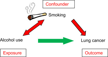
NoteConfounding factor
Let T represent a treatment (for example, alcohol use) and Y represent an outcome (for example, lung cancer).
A confounder is a variable that affects both T and Y, distorting the correlation between them. Using the example above, rich parents could be a confounder for breastfeeding and a baby’s health. Confounders can be a measured covariate (a feature) or an unmeasured variable we don’t know about, and they generally cause problems, as the relationship between T and Y is affected by data we cannot see. We commonly assume that all confounders are observed and adjusted for (this is also called ignorability).
Collinearity
Adding new terms to a regularized model often improves predictive performance.
So, as long as we’re at it, let’s add another variable to our lifetime earnings regression: \[
\widehat{\text{Earnings}} = \hat{\theta}_0 + \hat{\theta}_1 (\text{Has college degree}) + \hat{\theta}_2 (\text{Family wealth in dollars}) + \hat{\theta}_3 (\text{Has lived in a college town})
\]
Is adding this term appropriate if we want to make inferences about \(\hat{\theta}_1\)? Probably not.
Having a college degree and living in a college town are very highly correlated features. To the regression model, these features look very similar!
The regression model does not know that a college degree is more likely to change earnings than living in a college town. This is causal domain knowledge.
The fitting process of OLS minimizes RMSE (i.e., it maximizes predictive performance).
Because degree-status and living in a college town tend to have the same value, we could increase \(\hat{\theta}_1\) by \(\$X\) and decrease \(\hat{\theta}_3\) by \(\$X\) without changing the RMSE all that much.
So, the \(\hat{\theta}_1\) and \(\hat{\theta}_3\) coefficients will be sensitive to the training data (i.e., high variance).
This high variance does not harm predictive performance, but it does harm the validity of \(\hat{\theta}_1\) as a measure of the association between college degrees and lifetime earnings.
In general, if you want to make inferences about a parameter, don’t include features that are highly correlated with that parameter’s feature.
[Bonus Content]
How to perform causal inference?
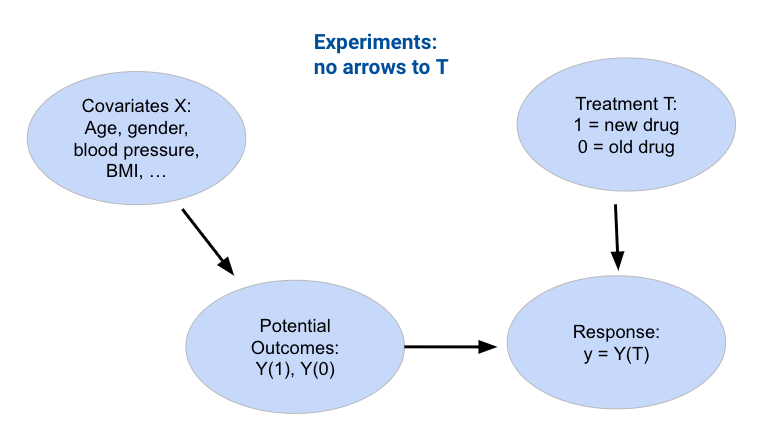
In a randomized experiment, participants are randomly assigned into two groups: treatment and control. A treatment is applied only to the treatment group. We assume ignorability and gather as many measurements as possible so that we can compare them between the control and treatment groups to determine whether or not the treatment has a true effect or is just a confounding factor.
However, often, randomly assigning treatments is impractical or unethical. For example, assigning a treatment of cigarettes to test the effect of smoking on the lungs would not only be impractical but also unethical.
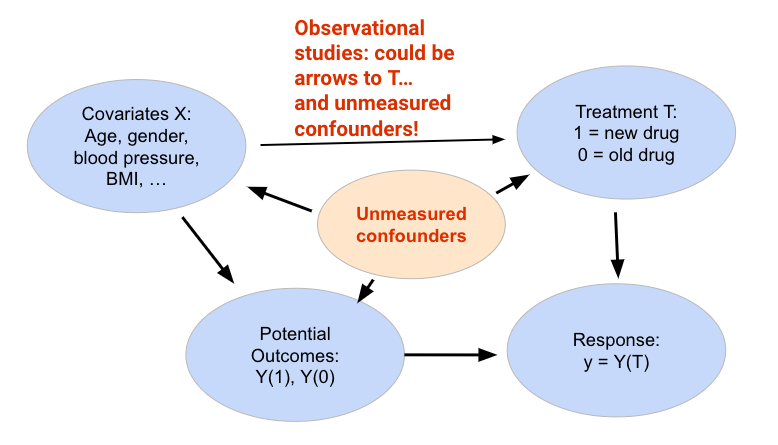
An alternative to bypass this issue is to utilize observational studies. This can be done by obtaining two participant groups separated based on some identified treatment variable. Unlike randomized experiments, however, we cannot assume ignorability here: the participants could have separated into two groups based on other covariates! In addition, there could also be unmeasured confounders.
Hypothesis Testing Through Bootstrap
We looked at a simple example of bootstrapping earlier, but now, let’s use bootstrapping to perform hypothesis testing. Recall that we use bootstrapping to compute approximate 95% confidence intervals for each \(\theta_i\). If the interval doesn’t contain 0, we reject the null hypothesis at the p=5% level. Otherwise, the data is consistent with the null, as the true parameter could possibly be 0.
To show an example of this hypothesis testing process, we’ll work with the snowy plover dataset throughout this section. The data are about the eggs and newly hatched chicks of the Snowy Plover. The data were collected at the Point Reyes National Seashore by a former student at Berkeley. Here’s a parent bird and some eggs.
Note that Egg Length and Egg Breadth (widest diameter) are measured in millimeters, and Egg Weight and Bird Weight are measured in grams. For reference, a standard paper clip weighs about one gram.
Code
import pandas as pdeggs = pd.read_csv("data/snowy_plover.csv")eggs.head(5)
egg_weight
egg_length
egg_breadth
bird_weight
0
7.4
28.80
21.84
5.2
1
7.7
29.04
22.45
5.4
2
7.9
29.36
22.48
5.6
3
7.5
30.10
21.71
5.3
4
8.3
30.17
22.75
5.9
Our goal will be to predict the weight of a newborn plover chick, which we assume follows the true relationship \(Y = f_{\theta}(x)\) below.
Note that for each \(i\), the parameter \(\theta_i\) is a fixed number, but it is unobservable. We can only estimate it. The random error \(\epsilon\) is also unobservable, but it is assumed to have expectation 0 and be independent and identically distributed across eggs.
Say we wish to determine if the egg_weight impacts the bird_weight of a chick – we want to infer if \(\theta_1\) is equal to 0.
First, we define our hypotheses:
Null hypothesis: the true parameter \(\theta_1\) is 0; any variation is due to random chance.
Alternative hypothesis: the true parameter \(\theta_1\) is not 0.
Next, we use our data to fit a model \(\hat{Y} = f_{\hat{\theta}}(x)\) that approximates the relationship above. This gives us the observed value of \(\hat{\theta}_1\) from our data.
from sklearn.linear_model import LinearRegressionimport numpy as npX = eggs[["egg_weight", "egg_length", "egg_breadth"]]Y = eggs["bird_weight"]model = LinearRegression()model.fit(X, Y)# This gives an array containing the fitted model parameter estimatesthetas = model.coef_# Put the parameter estimates in a nice table for viewingdisplay(pd.DataFrame( [model.intercept_] +list(model.coef_), columns=['theta_hat'], index=['intercept', 'egg_weight', 'egg_length', 'egg_breadth']))print("RMSE", np.mean((Y - model.predict(X)) **2))
theta_hat
intercept
-4.605670
egg_weight
0.431229
egg_length
0.066570
egg_breadth
0.215914
RMSE 0.04547085380275775
Our single sample of data gives us the value of \(\hat{\theta}_1=0.431\). To get a sense of how this estimate might vary if we were to draw different random samples, we will use bootstrapping. As a refresher, to construct a bootstrap sample, we will draw a resample from the collected data that:
Has the same sample size as the collected data
Is drawn with replacement (this ensures that we don’t draw the exact same sample every time!)
We draw a bootstrap sample, use this sample to fit a model, and record the result for \(\hat{\theta}_1\) on this bootstrapped sample. We then repeat this process many times to generate a bootstrapped empirical distribution of \(\hat{\theta}_1\). This gives us an estimate of what the true distribution of \(\hat{\theta}_1\) across all possible samples might look like.
# Set a random seed so you generate the same random sample as staff# In the "real world", we wouldn't do thisimport numpy as npnp.random.seed(1337)# Set the sample size of each bootstrap samplen =len(eggs)# Create a list to store all the bootstrapped estimatesestimates = []# Generate a bootstrap resample from `eggs` and find an estimate for theta_1 using this sample. # Repeat 10000 times.for i inrange(10000):# draw a bootstrap sample bootstrap_resample = eggs.sample(n, replace=True) X_bootstrap = bootstrap_resample[["egg_weight", "egg_length", "egg_breadth"]] Y_bootstrap = bootstrap_resample["bird_weight"]# use bootstrapped sample to fit a model bootstrap_model = LinearRegression() bootstrap_model.fit(X_bootstrap, Y_bootstrap) bootstrap_thetas = bootstrap_model.coef_# record the result for theta_1 estimates.append(bootstrap_thetas[0])# calculate the 95% confidence interval lower = np.percentile(estimates, 2.5, axis=0)upper = np.percentile(estimates, 97.5, axis=0)conf_interval = (lower, upper)conf_interval
(-0.25864811956848743, 1.1034243854204049)
Our bootstrapped 95% confidence interval for \(\theta_1\) is \([-0.259, 1.103]\). Immediately, we can see that 0 is indeed contained in this interval – this means that we cannot conclude that \(\theta_1\) is non-zero! More formally, we fail to reject the null hypothesis (that \(\theta_1\) is 0) at a 5% cutoff.
We can repeat this process to construct 95% confidence intervals for the other parameters of the model.
Something’s off here. Notice that 0 is included in the 95% confidence interval for every parameter of the model. Using the interpretation we outlined above, this would suggest that we can’t say for certain that any of the input variables impact the response variable! This makes it seem like our model can’t make any predictions – and yet, each model we fit in our bootstrap experiment above could very much make predictions of \(Y\).
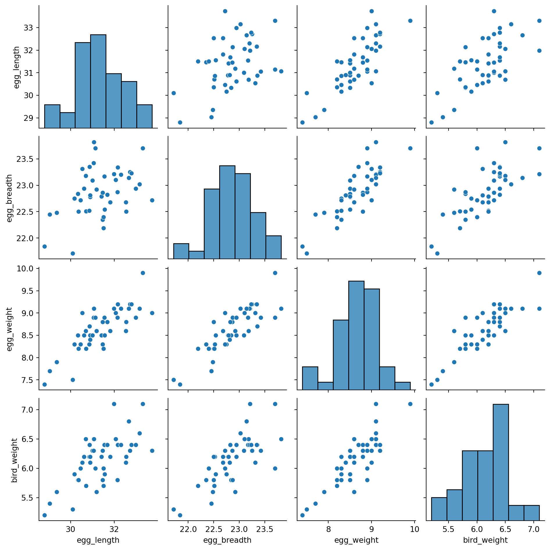
How can we explain this result? Think back to how we first interpreted the parameters of a linear model. We treated each \(\theta_i\) as a slope, where a unit increase in \(x_i\) leads to a \(\theta_i\) increase in \(Y\), if all other variables are held constant. It turns out that this last assumption is very important. If variables in our model are somehow related to one another, then it might not be possible to have a change in one of them while holding the others constant. This means that our interpretation framework is no longer valid! In the models we fit above, we incorporated egg_length, egg_breadth, and egg_weight as input variables. These variables are very likely related to one another – an egg with large egg_length and egg_breadth will likely be heavy in egg_weight. This means that the model parameters cannot be meaningfully interpreted as slopes.
To support this conclusion, we can visualize the relationships between our feature variables. Notice the strong positive association between the features.
Code
import seaborn as snssns.pairplot(eggs[["egg_length", "egg_breadth", "egg_weight", 'bird_weight']]);
This issue is known as collinearity, sometimes also called multicollinearity. Collinearity occurs when one feature can be predicted fairly accurately by a linear combination of the other features, which happens when one feature is highly correlated with the others.
Why is collinearity a problem? Its consequences span several aspects of the modeling process:
Inference: Slopes can’t be interpreted for an inference task.
Model Variance: If features strongly influence one another, even small changes in the sampled data can lead to large changes in the estimated slopes.
Unique Solution: If one feature is a linear combination of the other features, the design matrix will not be full rank, and \(\mathbb{X}^{\top}\mathbb{X}\) is not invertible. This means that least squares does not have a unique solution. See this section of Course Note 12 for more on this.
The take-home point is that we need to be careful with what features we select for modeling. If two features likely encode similar information, it is often a good idea to choose only one of them as an input variable.
A Simpler Model
Let us now consider a more interpretable model: we instead assume a true relationship using only egg weight:
from sklearn.linear_model import LinearRegressionX_int = eggs[["egg_weight"]]Y_int = eggs["bird_weight"]model_int = LinearRegression()model_int.fit(X_int, Y_int)# This gives an array containing the fitted model parameter estimatesthetas_int = model_int.coef_# Put the parameter estimates in a nice table for viewingpd.DataFrame({"theta_hat":[model_int.intercept_, thetas_int[0]]}, index=["theta_0", "theta_1"])
theta_hat
theta_0
-0.058272
theta_1
0.718515
Code
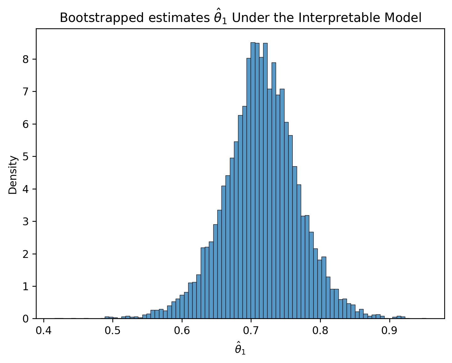
import matplotlib.pyplot as plt# Set a random seed so you generate the same random sample as staff# In the "real world", we wouldn't do thisnp.random.seed(1337)# Set the sample size of each bootstrap samplen =len(eggs)# Create a list to store all the bootstrapped estimatesestimates_int = []# Generate a bootstrap resample from `eggs` and find an estimate for theta_1 using this sample. # Repeat 10000 times.for i inrange(10000): bootstrap_resample_int = eggs.sample(n, replace=True) X_bootstrap_int = bootstrap_resample_int[["egg_weight"]] Y_bootstrap_int = bootstrap_resample_int["bird_weight"] bootstrap_model_int = LinearRegression() bootstrap_model_int.fit(X_bootstrap_int, Y_bootstrap_int) bootstrap_thetas_int = bootstrap_model_int.coef_ estimates_int.append(bootstrap_thetas_int[0])plt.figure(dpi=120)sns.histplot(estimates_int, stat="density")plt.xlabel(r"$\hat{\theta}_1$")plt.title(r"Bootstrapped estimates $\hat{\theta}_1$ Under the Interpretable Model");
Notice how the interpretable model performs almost as well as our other model:
Code
from sklearn.metrics import mean_squared_errorrmse = mean_squared_error(Y, model.predict(X))rmse_int = mean_squared_error(Y_int, model_int.predict(X_int))print(f'RMSE of Original Model: {rmse}')print(f'RMSE of Interpretable Model: {rmse_int}')
RMSE of Original Model: 0.04547085380275775
RMSE of Interpretable Model: 0.046493941375556846
Yet, the confidence interval for the true parameter \(\theta_{1}\) does not contain zero.