Dissect Singular Value Decomposition (SVD) and use it to calculate principal components
Develop a deeper understanding of how to interpret Principal Component Analysis (PCA)
See applications of PCA in some real-world contexts
25.1 PCA as Loss Minimization
We often work with high-dimensional data that contain many columns/features. Given all these dimensions, this data can be difficult to visualize and model. However, not all the data in this high-dimensional space is useful — there could be repeated features or outliers that make the data seem more complex than it really is. The most concise representation of high-dimensional data is its intrinsic dimension.
Our goal with this lecture is to use dimensionality reduction to find the intrinsic dimension of a high-dimensional dataset. In other words, we want to find a smaller set of new features/columns that approximates the original data well without losing that much information. This is especially useful because this smaller set of features allows us to better visualize the data and do EDA to understand which modeling techniques would fit the data well. Let’s treat this as a matrix factorization problem, and review what we covered in the previous lecture.
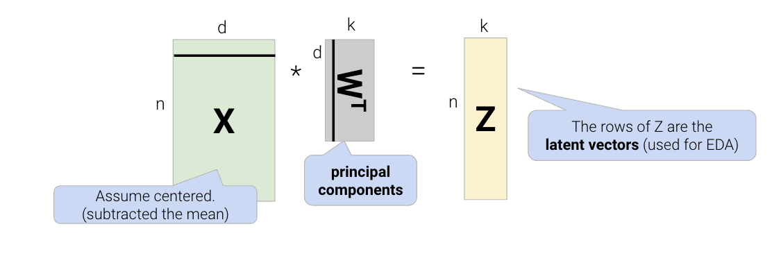
In order to find the intrinsic dimension of a high-dimensional dataset, we’ll use techniques from linear algebra. Suppose we have a high-dimensional dataset, \(X\), that has \(n\) rows and \(d\) columns. We want to factor (split) \(X \in \mathbb{R}^{n \times d}\) into two matrices, \(Z \in \mathbb{R}^{n \times k}\) and \(W \in \mathbb{R}^{k \times d}\): \[X \approx ZW\]
We can reframe this problem as a loss function, minimizing difference between \(X\) and \(ZW\): \[L(Z, W) = \frac{1}{n}\sum_{i=1}^{n}||X_i - Z_i W||^2\]
Breaking down the variables in this formula:
\(X_i\): A row vector from the original data matrix \(X\), which we can assume is centered to a mean of 0.
\(Z_i\): A row vector from the lower-dimension matrix \(Z\). The rows of \(Z\) are also known as latent vectors and are used for EDA.
\(W\): The rows of \(W\) are the principal components. We constrain our model so that \(W\) is a row-orthonormal matrix (e.g., \(WW^T = I\)).
Using calculus and optimization techniques (take EECS 127 if you’re interested!), we find that this loss is minimized when \[Z = XW^T\] The proof for this is out of scope for Data 100, but for those who are interested, we:
Use Lagrangian multipliers to introduce the orthonormality constraint on \(W\).
Took the derivative with respect to \(W\) (which requires vector calculus) and solve for 0.
Take a look at the previous lecture note for the full proof. This gives us a very cool result of \[\Sigma w^T = \lambda w^T\]
\(\Sigma\) is the covariance matrix of \(X\). The equation above implies that:
\(w\) is a unitary eigenvector of the covariance matrix \(\Sigma\). In other words, its norm is equal to 1: \(||w||^2 = ww^T = 1\).
The error is minimized when \(w\) is the eigenvector with the largest eigenvalue\(\lambda\).
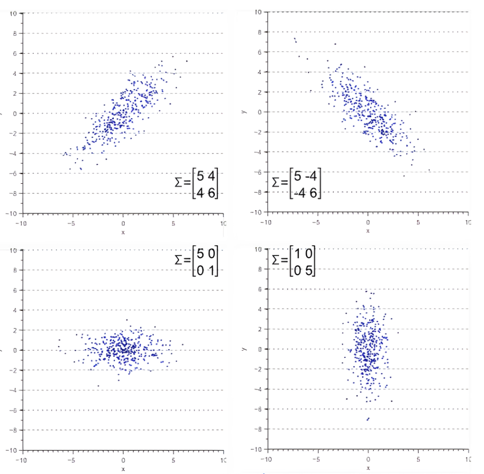
Tip[Linear Algebra Review] Covariance Matrix
Covariance matrix defines spread (variance) and orientation (covariance) of our data.
Geometrically, we can represent the covariance matrix with a vector, pointing into the direction of the largest spread of the data, and whose magnitude equals the spread (variance) in this direction.
Diagonal elements: variance of data along each dimension.
Off-diagonal elements: covariance of different dimensions.
This tells us that the principal components (rows of \(W\)) are the eigenvectors with the largest eigenvalues of the covariance matrix \(\Sigma\). Thus, principal components represent the directions of maximum variance in the data. We can construct the latent factors, or the \(Z\) matrix, by projecting the centered data \(X\) onto the principal component vectors, \(W^T\).
But how do we compute the eigenvectors of \(\Sigma\)? Let’s dive into SVD to answer this question.
25.2 Singular Value Decomposition (SVD)
Singular value decomposition (SVD) is an important concept in linear algebra. Since this class requires a linear algebra course (MATH 54, MATH 56, or EECS 16A) as a pre/co-requisite, we assume you have taken or are taking a linear algebra course, so we won’t explain SVD in its entirety. In particular, we will not prove why SVD is a valid decomposition of rectangular matrices.
We will not dive deep into the theory and details of SVD. Instead, we will only cover what is needed for a data science interpretation. If you’d like more information, check out EECS 16B Note 14 and EECS 16B Note 15.
Tip[Linear Algebra Review] Orthonormality
Orthonormal is a combination of two words: orthogonal and normal.
When we say the columns of a matrix are orthonormal, we know that:
The columns are all orthogonal to each other (all pairs of columns have a dot product of zero)
All columns are unit vectors (the length of each column vector is 1)
Orthonormal matrices have a few important properties:
Orthonormal inverse: If an \(m \times n\) matrix \(Q\) has orthonormal columns, \(QQ^T= Iₘ\) and \(Q^TQ=Iₙ\).
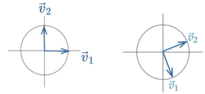
Rotation of coordinates: The linear transformation represented by an orthonormal matrix is often a rotation (and less often a reflection). We can imagine columns of the matrix as where the unit vectors of the original space will land.
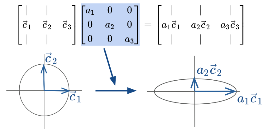
Tip[Linear Algebra Review] Diagonal Matrices
Diagonal matrices are square matrices with non-zero values on the diagonal axis and zeros everywhere else.
Right-multiplied diagonal matrices scale each column up or down by a constant factor. Geometrically, this transformation can be viewed as scaling the coordinate system.
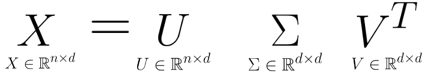
Singular value decomposition (SVD) describes a matrix \(X\)’s decomposition into three matrices: \[ X = U S V^T \]
Let’s break down each of these terms one by one.
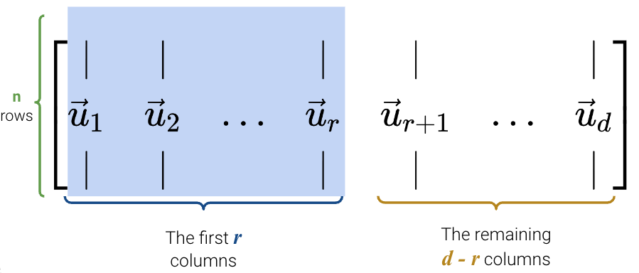
25.2.1\(U\)
\(U\) is an \(n \times d\) matrix: \(U \in \mathbb{R}^{n \times d}\).
Its columns are orthonormal.
\(\vec{u_i}^T\vec{u_j} = 0\) for all pairs \(i, j\).
All vectors \(\vec{u_i}\) are unit vectors where \(|| \vec{u_i} || = 1\) .
Columns of \(U\) are called the left singular vectors and are eigenvectors of \(XX^T\).
\(UU^T = I_n\) and \(U^TU = I_d\).
We can think of \(U\) as a rotation.
Here is a proof that \(U\) consists of the eigenvectors of \(XX^T\): \[\begin{align}
XX^T &= USV^T (USV^T)^T \\
&= USV^T V S^T U^T \\
&= USS^T U^T
\end{align}\]
Now right multiply by \(U\): \[\begin{align}
XX^T U &= US S^T U^T U \\
&= US S^T
\end{align}\]
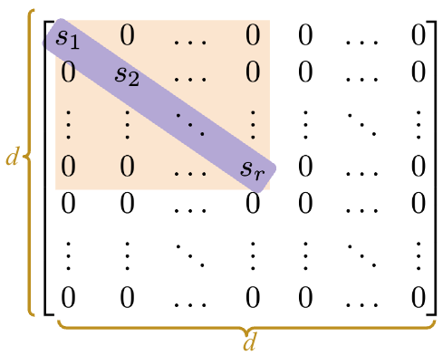
25.2.2\(S\)
\(S\) is a \(d \times d\) matrix: \(S \in \mathbb{R}^{d \times d}\).
The majority of the matrix is zero.
It has \(r\)non-zerosingular values, and \(r\) is the rank of \(X\). Note that rank \(r \leq d\).
Diagonal values (singular values\(s_1, s_2, ... s_r\)), are non-negative ordered from largest to smallest: \(s_1 \ge s_2 \ge ... \ge s_r > 0\).
We can think of \(S\) as a scaling operation.
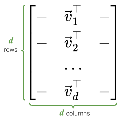
25.2.3\(V^T\)
\(V^T\) is an \(d \times d\) matrix: \(V \in \mathbb{R}^{d \times d}\).
Columns of \(V\) are orthonormal, so the rows of \(V^T\) are orthonormal.
Columns of \(V\) are called the right singular vectors, and similarly to \(U\), are eigenvectors of \(X^TX\).
\(VV^T = V^TV = I_d\)
We can think of \(V\) as a rotation.
Just like before, here is a proof that \(V\) consists of the eigenvectors of \(X^TX\): \[\begin{align}
X^TX &= (USV^T)^T USV^T \\
&= V S^T U^T USV^T \\
&= VS^TS V^T
\end{align}\]
Now right multiply by \(V\): \[\begin{align}
X^TX V &= VS^T S V^T V \\
&= VS^T S
\end{align}\]
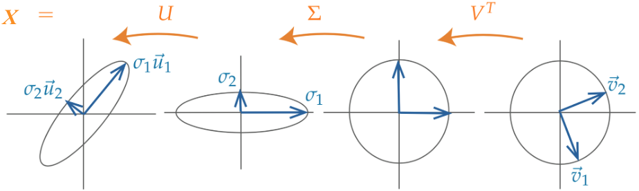
TipSVD: Geometric Perspective
We’ve seen that \(U\) and \(V\) represent rotations, and \(S\) represents scaling. Therefore, SVD says that any matrix can be decomposed into a rotation, then a scaling, and another rotation.
25.2.4 SVD in NumPy
For this demo, we’ll work with a rectangular dataset containing \(n=100\) rows and \(d=4\) columns.
Code
import pandas as pdimport seaborn as snsimport matplotlib.pyplot as pltimport numpy as npnp.random.seed(23) # kallistiplt.rcParams["figure.figsize"] = (4, 4)plt.rcParams["figure.dpi"] =150sns.set()rectangle = pd.read_csv("data/rectangle_data.csv")rectangle.head(5)
width
height
area
perimeter
0
8
6
48
28
1
2
4
8
12
2
1
3
3
8
3
9
3
27
24
4
9
8
72
34
In NumPy, the SVD decomposition function can be called with np.linalg.svd (documentation). There are multiple versions of SVD; to get the version that we will follow, we need to set the full_matrices parameter to False.
U, S, Vt = np.linalg.svd(rectangle, full_matrices=False)
First, let’s examine U. As we can see, it’s dimensions are \(n \times d\).
U.shape
(100, 4)
The first 5 rows of U are shown below.
pd.DataFrame(U).head(5)
0
1
2
3
0
-0.155151
0.064830
-0.029935
0.967868
1
-0.038370
-0.089155
0.062019
-0.151231
2
-0.020357
-0.081138
0.058997
0.003355
3
-0.101519
-0.076203
-0.148160
0.006977
4
-0.218973
0.206423
0.007274
-0.042254
\(S\) is a little different in NumPy. Since the only useful values in the diagonal matrix \(S\) are the singular values on the diagonal axis, only those values are returned and they are stored in an array.
Our rectangle_data has a rank of \(3\), so we should have 3 non-zero singular values, sorted from largest to smallest.
It seems like we have 4 non-zero values instead of 3, but notice that the last value is so small (\(10^{-15}\)) that it’s practically \(0\). Hence, we can round the values to get 3 singular values.
Finally, we can see that Vt is indeed a \(d \times d\) matrix.
Vt.shape
(4, 4)
pd.DataFrame(Vt)
0
1
2
3
0
-0.146436
-0.129942
-8.100201e-01
-0.552756
1
-0.192736
-0.189128
5.863482e-01
-0.763727
2
-0.704957
0.709155
7.951614e-03
0.008396
3
-0.666667
-0.666667
-8.701245e-17
0.333333
To check that this SVD is a valid decomposition, we can reverse it and see if it matches our original table (it does, yay!).
pd.DataFrame(U @ Sm @ Vt).head(5)
0
1
2
3
0
8.0
6.0
48.0
28.0
1
2.0
4.0
8.0
12.0
2
1.0
3.0
3.0
8.0
3
9.0
3.0
27.0
24.0
4
9.0
8.0
72.0
34.0
25.3 PCA with SVD
Principal Component Analysis (PCA) and Singular Value Decomposition (SVD) can be easily mixed up, especially when you have to keep track of so many acronyms. Here is a quick summary:
SVD: a linear algebra algorithm that splits a matrix into 3 component parts.
PCA: a data science procedure used for dimensionality reduction that uses SVD as one of the steps.
Let’s summarize first the steps to obtain Principal Components via SVD:
Center the data matrix\(X\) by subtracting the mean of each attribute column.
The Scikit-Learn PCA code does this automatically
X = X - np.mean(X, axis = 0)
You should also consider standardizing your data (ensure unit variance on each dimension)
The Scikit-Learn PCA code does not do this, but you should standardize your data if features have vastly different ranges.
You should not standardize your data if the units are all the same and the differences in variability across dimensions is meaningful (e.g., everything is in the same units)
To find the \(k\)principal components:
Compute the SVD of the data matrix (\(X = U{S}V^{T}\)).
The first \(k\) columns of \(V\) contain the \(k\)principal components of \(X\). The \(k\)-th column of \(V\) is also known as the \(k\)-th principal component and corresponds to the \(k\)-th largest singular value of \(X\).
25.3.1 Deriving Principal Components From SVD
After centering the original data matrix \(X\) so that each column has a mean of 0, we find its SVD: \[ X = U S V^T \]
Because \(X\) is centered, the covariance matrix of \(X\), \(\Sigma\), is equal to \(\frac{1}{n}X^T X\). Rearranging this equation, we get
\[
\begin{align}
\Sigma &= \frac{1}{n}X^T X \\
&= \frac{1}{n}(U S V^T)^T U S V^T \\
&= \frac{1}{n}V S^T U^T U S V^T & \text{U is orthonormal, so $U^T U = I$} \\
&= \frac{1}{n}V S^2 V^T
\end{align}
\]
Multiplying both sides by \(V\), we get
\[
\begin{align}
\Sigma V &= \frac{1}{n}VS^2 V^T V \\
&= \frac{1}{n}V S^2
\end{align}
\]
This shows that the columns of \(V\) are the eigenvectors of the covariance matrix \(\Sigma\) and, therefore, the principal components. Additionally, the squared singular values \(S^2\) (divided by \(n\)) are the eigenvalues of \(\Sigma\).
We’ve now shown that the first \(k\) columns of \(V\) (equivalently, the first \(k\) rows of \(V^{T}\)) are the first k principal components of \(X\). We can use them to construct the latent vector representation of \(X\), \(Z\), by projecting \(X\) onto the principal components.
We also have a second way of computing \(Z\) as follows:
\[
\begin{align}
Z &= X V \\
&= USV^T V \\
&= U S
\end{align}
\]
\[Z = XV = US\]
In other words, we can construct \(X\)’s’ latent vector representation \(Z\) through:
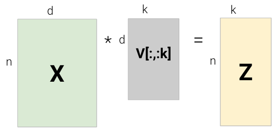
Projecting \(X\) onto the first \(k\) columns of \(V\), \(V[:, :k]\)
Multiplying the first \(k\) columns of U and the first \(k\) rows of S
Using \(Z\), we can approximately recover the centered \(X\) matrix by multiplying \(Z\) by \(V^T\): \[ Z V^T = XV V^T = USV^T = X\]
If we choose a k that is less than the rank of X then we will only recover X approximately. Note that to recover the original (uncentered) \(X\) matrix, we would also need to add back the mean.
Tip[Summary] Terminology
Note: The notation used for PCA this semester differs from previous semesters a bit. Please pay careful attention to the terminology presented in this note.
To summarize the terminology and concepts we’ve covered so far:
Principal Component: The columns of \(V\) . These vectors specify the principal coordinate system and represent the directions along which the most variance in the data is captured.
Latent Vector Representation of \(X\): The projection of our data matrix \(X\) onto the principal components, \(Z = XV = US\) (as denoted in lecture). The columns of Z are called latent factors or component scores. In previous semesters, the terminology was different and this was termed the principal components of \(X\). In other classes, the term principal coordinate is also used.
\(S\) (as in SVD): The diagonal matrix containing all the singular values of \(X\).
\(\Sigma\): The covariance matrix of \(X\). Assuming \(X\) is centered, \(\Sigma = \frac{1}{n}X^T X\). In previous semesters, the singular value decomposition of \(X\) was written out as \(X = U{\Sigma}V^T\), but we now use \(X = USV^T\). Note the difference between \(\Sigma\) in that context compared to this semester.
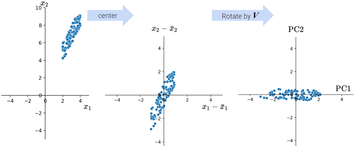
25.3.2 PCA Visualization
As we discussed above, when conducting PCA, we first center the data matrix\(X\) and then rotate it such that the direction with the most variation (i.e., the direction that is most spread out) aligns with the x-axis.
In particular, the elements of each principal component or column of \(V\) (row of \(V^{T}\)) rotate the original feature vectors, projecting \(X\) onto the principal components. The first column of \(V\) indicates how each feature contributes (e.g. positive, negative, etc.) to the first latent factor; it essentially assigns “weights” to each feature.
Coupled together, this interpretation also allows us to understand that:
The principal components are all orthogonal to each other because the columns of \(V\) are orthonormal.
Principal components are axis-aligned. That is, if you plot two PCs on a 2D plane, one will lie on the x-axis and the other on the y-axis.
The latent factors are obtained by projecting X onto the principal components.
25.3.3 Code Demo
Let’s now walk through an example where we compute PCA using SVD. In order to get the first \(k\) principal components from an \(n \times d\) matrix \(X\), we:
Center \(X\) by subtracting the mean from each column. Notice how we specify axis=0 so that the mean is computed per column.
Get the Singular Value Decomposition of the centered \(X\): \(U\), \(S\) and \(V^T\)
U, S, Vt = np.linalg.svd(centered_df, full_matrices=False)Sm = pd.DataFrame(np.diag(np.round(S, 1)))
Take the first \(k\) columns of \(V\). These are the first \(k\) principal components of \(X\).
two_PCs = Vt.T[:, :2]pd.DataFrame(two_PCs).head()
0
1
0
-0.098631
0.668460
1
-0.072956
-0.374186
2
-0.931226
-0.258375
3
-0.343173
0.588548
25.4 Centering Data and Computing Variance
We define the total variance of a data matrix as the sum of variances of attributes. The principal components are a low-dimension representation that capture as much of the original data’s total variance as possible. Formally, the \(i\)-th singular value tells us the component score, or how much of the data variance is captured by the \(i\)-th principal component. Assuming the number of datapoints is \(n\):
We often plot the first two principal components using a scatter plot, with PC1 on the \(x\)-axis and PC2 on the \(y\)-axis. This is often called a PCA plot.
If the first two singular values are large and all others are small, then two dimensions are enough to describe most of what distinguishes one observation from another. If not, a PCA plot omits a lot of information.
PCA plots help us assess similarities between our data points and if there are any clusters in our dataset. Here is one example:
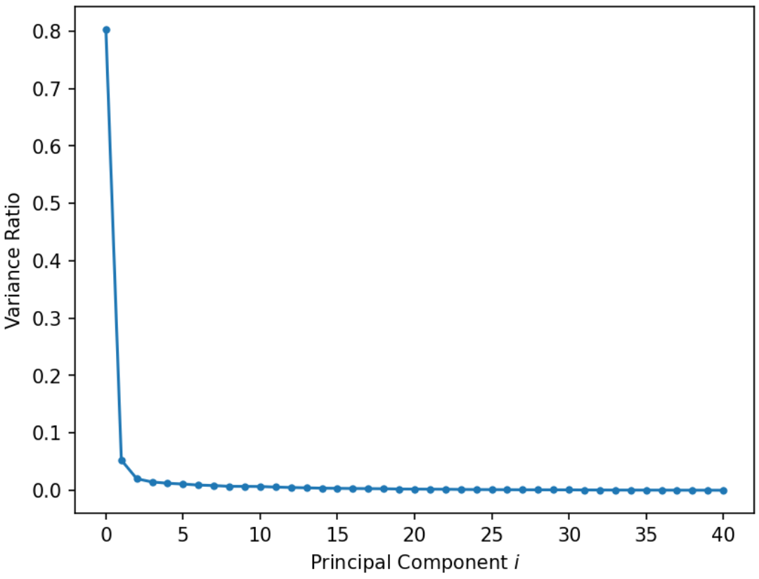
25.5.2 Scree Plots
A scree plot shows the variance ratio captured by each principal component, with the largest variance ratio first. Recall that we could use each singular value to determine the component score:
Therefore, the total variance is the sum of all component scores: \[\text{Total Variance} = \sum_{i=1}^{k} \frac{{s_i}^2}{N}\]
Then the variance ratio, or the proportion of fraction of total variance represented by a single principal component is the following: \[\text{Variance Ratio of Principal Component j} = \frac{\frac{{s_j}^2}{N}}{\sum_{i=1}^{k} \frac{{s_i}^2}{N}} = \frac{{s_j}^2}{\sum_{i=1}^{k} {s_i}^2}\]
In other words, the variance ratio is a principal component’s singular value squared divided by the sum of all singular values squared. Scree plots can help us visually determine the number of dimensions needed to describe the data reasonably. The singular values that fall in the region of the plot after a large drop-off correspond to principal components that are not needed to describe the data since they explain a relatively low proportion of the total variance of the data. This point where adding more principal components results in diminishing returns is called the “elbow” and is the point just before the line flattens out. Using this “elbow method”, we can see that the elbow is at the second principal component, so two dimensions are enough to describe most of what distinguishes one observation from another. If this was not the case, then a PCA scatter plot is omitting lots of information.
Interpreting this graph, first principal component explains 80% of the total variance in the data.
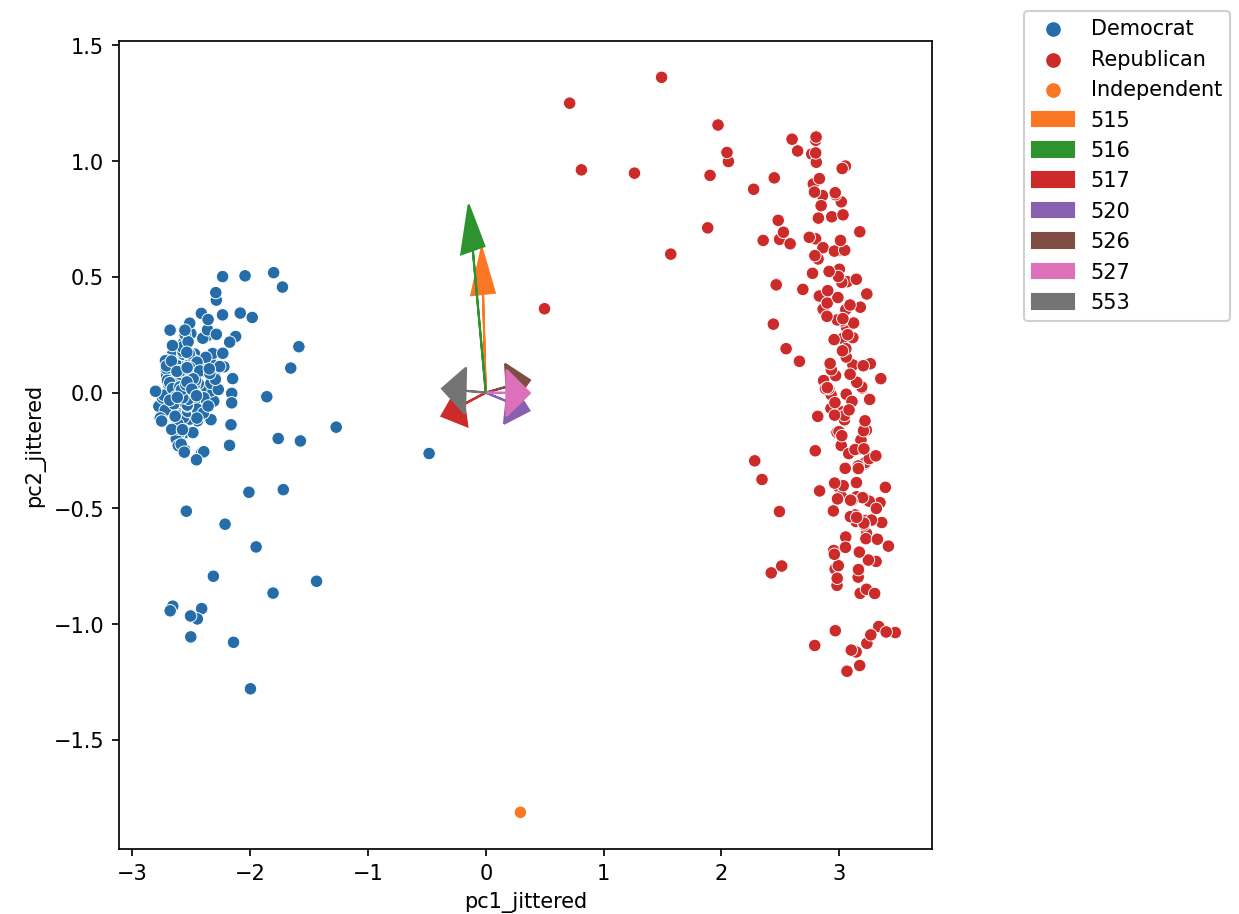
25.5.3 Biplots
Biplots superimpose the directions onto the plot of PC1 vs. PC2, where vector \(j\) corresponds to the direction for feature \(j\) (e.g., \(v_{1j}, v_{2j}\)). There are several ways to scale biplot vectors — in this course, we plot the direction itself. For other scalings, which can lead to more interpretable directions/loadings, see SAS biplots.
Through biplots, we can interpret how features correlate with the principal components shown: positively, negatively, or not much at all.
The directions of the arrow are (\(v_1\), \(v_2\)), where \(v_1\) and \(v_2\) are how that specific feature column contributes to PC1 and PC2, respectively. \(v_1\) and \(v_2\) are elements of the first and second columns of \(V\), respectively (i.e., the first two rows of \(V^T\)).
Say we were considering feature 3, and say that was the purple arrow labeled “520” here (pointing bottom right).
\(v_1\) and \(v_2\) are the third elements of the respective columns in \(V\). They are scale feature 3’s column vector in the linear transformation to PC1 and PC2, respectively.
Here, we would infer that \(v_1\) (in the \(x\)/PC1-direction) is positive, meaning that a linear increase in feature 3 would correspond to a linear increase of PC1, meaning feature 3 and PC1 are positively correlated.
\(v_2\) (in the \(y\)/pc2-direction) is negative, meaning a linear increase in feature 3 would correspond to a linear decrease in PC2, meaning feature 3 and PC2 are negatively correlated.
25.6 Example: House of Representatives Voting
Let’s examine how the House of Representatives (of the 116th Congress, 1st session) voted in the month of September 2019.
Specifically, we’ll look at the records of Roll call votes. From the U.S. Senate (link): roll call votes occur when a representative or senator votes “yea” or “nay” so that the names of members voting on each side are recorded. A voice vote is a vote in which those in favor or against a measure say “yea” or “nay,” respectively, without the names or tallies of members voting on each side being recorded.
Code
import pandas as pdimport seaborn as snsimport matplotlib.pyplot as pltimport numpy as npimport yamlfrom datetime import datetimeimport plotly.express as pximport plotly.graph_objects as govotes = pd.read_csv("data/votes.csv")votes = votes.astype({"roll call": str})votes.head()
chamber
session
roll call
member
vote
0
House
1
555
A000374
Not Voting
1
House
1
555
A000370
Yes
2
House
1
555
A000055
No
3
House
1
555
A000371
Yes
4
House
1
555
A000372
No
Suppose we pivot this table to group each legislator and their voting pattern across every (roll call) vote in this month. We mark 1 if the legislator voted Yes (“yea”), and 0 otherwise (“No”, “nay”, no vote, speaker, etc.).
Do legislators’ roll call votes show a relationship with their political party?
25.6.1 PCA with SVD
While we could consider loading information about the legislator, such as their party, and see how this relates to their voting pattern, it turns out that we can do a lot with PCA to cluster legislators by how they vote. Let’s calculate the principal components using the SVD method.
It looks like this graph plateaus after the third principal component, so our “elbow” is at PC3, and most of the variance is captured by just the first three principal components. Let’s use these PCs to visualize the latent vector representation of \(X\)!
# Calculate the latent vector representation (US or XV)# using the first 3 principal componentsvote_2d = pd.DataFrame(index=vote_pivot_centered.index)vote_2d[["z1", "z2", "z3"]] = (u * s)[:, :3]# Plot the latent vector representationfig = px.scatter_3d(vote_2d, x='z1', y='z2', z='z3', title='Vote Data', width=800, height=600)fig.update_traces(marker=dict(size=5))
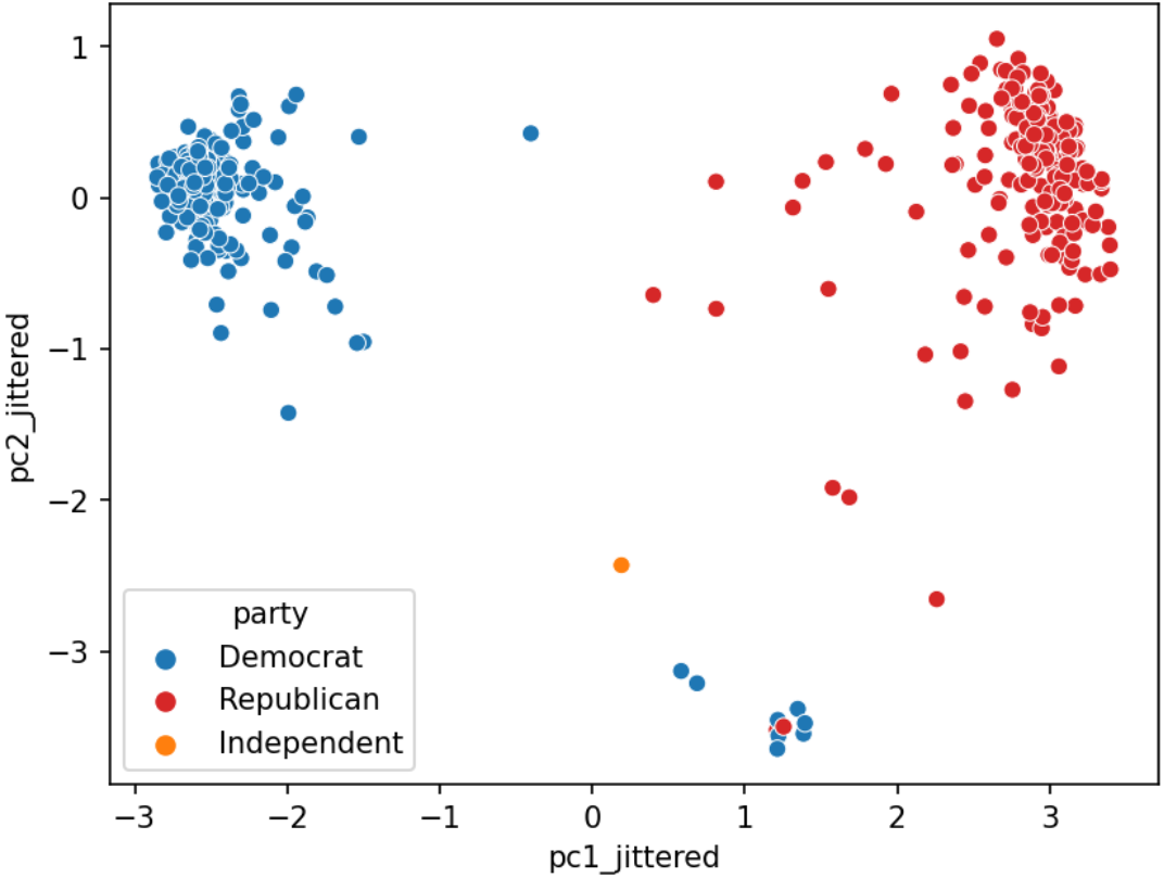
Baesd on the plot above, it looks like there are two clusters of datapoints. What do you think this corresponds to?
By incorporating member information (source), we can augment our graph with biographic data like each member’s party and gender.
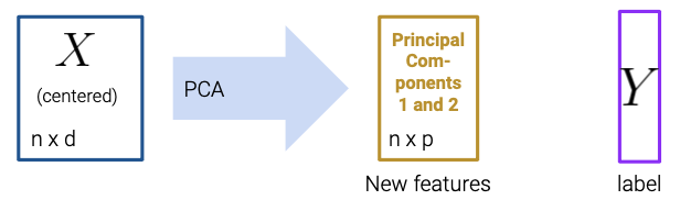
As shown in the demo, the primary goal of PCA is to transform observations from high-dimensional data down to low dimensions through linear transformations.
25.7 Example: Image Classification
In machine learning, PCA is often used as a preprocessing step prior to training a supervised model.
Let’s explore how PCA is useful for building an image classification model based on the Fashion-MNIST dataset, a dataset containing images of articles of clothing; these images are gray scale with a size of 28 by 28 pixels. The copyright for Fashion-MNIST is held by Zalando SE. Fashion-MNIST is licensed under the MIT license.
First, we’ll load in the data.
Code
import requestsfrom pathlib import Pathimport timeimport gzipimport osimport numpy as npimport plotly.express as pxdef fetch_and_cache(data_url, file, data_dir="data", force=False):""" Download and cache a url and return the file object. data_url: the web address to download file: the file in which to save the results. data_dir: (default="data") the location to save the data force: if true the file is always re-downloaded return: The pathlib.Path object representing the file. """ data_dir = Path(data_dir) data_dir.mkdir(exist_ok=True) file_path = data_dir / Path(file)# If the file already exists and we want to force a download then# delete the file first so that the creation date is correct.if force and file_path.exists(): file_path.unlink()if force ornot file_path.exists():print("Downloading...", end=" ") resp = requests.get(data_url)with file_path.open("wb") as f: f.write(resp.content)print("Done!") last_modified_time = time.ctime(file_path.stat().st_mtime)else: last_modified_time = time.ctime(file_path.stat().st_mtime)print("Using cached version that was downloaded (UTC):", last_modified_time)return file_pathdef head(filename, lines=5):""" Returns the first few lines of a file. filename: the name of the file to open lines: the number of lines to include return: A list of the first few lines from the file. """from itertools import islicewithopen(filename, "r") as f:returnlist(islice(f, lines))def load_data():""" Loads the Fashion-MNIST dataset. This is a dataset of 60,000 28x28 grayscale images of 10 fashion categories, along with a test set of 10,000 images. This dataset can be used as a drop-in replacement for MNIST. The classes are: | Label | Description | |:-----:|-------------| | 0 | T-shirt/top | | 1 | Trouser | | 2 | Pullover | | 3 | Dress | | 4 | Coat | | 5 | Sandal | | 6 | Shirt | | 7 | Sneaker | | 8 | Bag | | 9 | Ankle boot | Returns: Tuple of NumPy arrays: `(x_train, y_train), (x_test, y_test)`. **x_train**: uint8 NumPy array of grayscale image data with shapes `(60000, 28, 28)`, containing the training data. **y_train**: uint8 NumPy array of labels (integers in range 0-9) with shape `(60000,)` for the training data. **x_test**: uint8 NumPy array of grayscale image data with shapes (10000, 28, 28), containing the test data. **y_test**: uint8 NumPy array of labels (integers in range 0-9) with shape `(10000,)` for the test data. Example: (x_train, y_train), (x_test, y_test) = fashion_mnist.load_data() assert x_train.shape == (60000, 28, 28) assert x_test.shape == (10000, 28, 28) assert y_train.shape == (60000,) assert y_test.shape == (10000,) License: The copyright for Fashion-MNIST is held by Zalando SE. Fashion-MNIST is licensed under the [MIT license]( https://github.com/zalandoresearch/fashion-mnist/blob/master/LICENSE). """ dirname = os.path.join("datasets", "fashion-mnist") base ="https://storage.googleapis.com/tensorflow/tf-keras-datasets/" files = ["train-labels-idx1-ubyte.gz","train-images-idx3-ubyte.gz","t10k-labels-idx1-ubyte.gz","t10k-images-idx3-ubyte.gz", ] paths = []for fname in files: paths.append(fetch_and_cache(base + fname, fname))# paths.append(get_file(fname, origin=base + fname, cache_subdir=dirname))with gzip.open(paths[0], "rb") as lbpath: y_train = np.frombuffer(lbpath.read(), np.uint8, offset=8)with gzip.open(paths[1], "rb") as imgpath: x_train = np.frombuffer(imgpath.read(), np.uint8, offset=16).reshape(len(y_train), 28, 28 )with gzip.open(paths[2], "rb") as lbpath: y_test = np.frombuffer(lbpath.read(), np.uint8, offset=8)with gzip.open(paths[3], "rb") as imgpath: x_test = np.frombuffer(imgpath.read(), np.uint8, offset=16).reshape(len(y_test), 28, 28 )return (x_train, y_train), (x_test, y_test)
Code
class_names = ["T-shirt/top","Trouser","Pullover","Dress","Coat","Sandal","Shirt","Sneaker","Bag","Ankle boot",]class_dict = {i: class_name for i, class_name inenumerate(class_names)}(train_images, train_labels), (test_images, test_labels) = load_data()print("Training images", train_images.shape)print("Test images", test_images.shape)rng = np.random.default_rng(42)n =5000sample_idx = rng.choice(np.arange(len(train_images)), size=n, replace=False)# Invert and normalize the images so they look betterimg_mat =-1* train_images[sample_idx].astype(np.int16)img_mat = (img_mat - img_mat.min()) / (img_mat.max() - img_mat.min())images = pd.DataFrame( {"images": img_mat.tolist(),"labels": train_labels[sample_idx],"class": [class_dict[x] for x in train_labels[sample_idx]], })
Using cached version that was downloaded (UTC): Fri Aug 29 11:47:08 2025
Using cached version that was downloaded (UTC): Fri Aug 29 11:47:08 2025
Using cached version that was downloaded (UTC): Fri Aug 29 11:47:08 2025
Using cached version that was downloaded (UTC): Fri Aug 29 11:47:08 2025
Training images (60000, 28, 28)
Test images (10000, 28, 28)
Let’s see what some of the images contained in this dataset look like.
Code
def show_images(images, ncols=5, max_images=30):# conver the subset of images into a n,28,28 matrix for facet visualization img_mat = np.array(images.head(max_images)["images"].to_list()) fig = px.imshow( img_mat, color_continuous_scale="gray", facet_col=0, facet_col_wrap=ncols, height=220*int(np.ceil(len(images) / ncols)), ) fig.update_layout(coloraxis_showscale=False)# Extract the facet number and convert it back to the class label. fig.for_each_annotation(lambda a: a.update(text=images.iloc[int(a.text.split("=")[-1])]["class"]) )return figfig = show_images(images.groupby("class", as_index=False).sample(2), ncols=6)fig.show()
Let’s break this down further and look at it by class, or the category of clothing:
As we can see, each 28x28 pixel image is labelled by the category of clothing it belongs to. Us humans can very easily look at these images and identify the type of clothing being displayed, even if the image is a little blurry. However, this task is less intuitive for machine learning models. To illustrate this, let’s take a small sample of the training data to see how the images above are represented in their raw format:
Code
images.head()
images
labels
class
0
[[1.0, 1.0, 1.0, 1.0, 1.0, 1.0, 1.0, 1.0, 1.0,...
3
Dress
1
[[1.0, 1.0, 1.0, 1.0, 1.0, 1.0, 1.0, 1.0, 1.0,...
4
Coat
2
[[1.0, 1.0, 1.0, 1.0, 1.0, 1.0, 1.0, 1.0, 1.0,...
0
T-shirt/top
3
[[1.0, 1.0, 1.0, 1.0, 1.0, 0.996078431372549, ...
2
Pullover
4
[[1.0, 1.0, 1.0, 1.0, 1.0, 1.0, 1.0, 1.0, 1.0,...
1
Trouser
Each row represents one image. Every image belongs to a "class" of clothing with it’s enumerated "label". In place of a typically displayed image, the raw data contains a 28x28 2D array of pixel values; each pixel value is a float between 0 and 1. If we just focus on the images, we get a 3D matrix. You can think of this as a matrix containing 2D images.
X = np.array(images["images"].to_list())X.shape
(5000, 28, 28)
However, we’re not used to working with 3D matrices for our training data X. Typical training data expects a vector of features for each datapoint, not a matrix per datapoint. We can reshape our 3D matrix so that it fits our typical training data by “unrolling” the the 28x28 pixels into a single row vector containing 28*28 = 784 dimensions.
X = X.reshape(X.shape[0], -1)X.shape
(5000, 784)
What we have now is 5000 datapoints that each have 784 features. That’s a lot of features! Not only would training a model on this data take a very long time, it’s also very likely that our matrix is linearly independent. PCA is a very good strategy to use in situations like these when there are lots of features, but we want to remove redundant information.
25.7.2 PCA with sklearn
To perform PCA, let’s begin by centering our data.
X = X - X.mean(axis=0)
We can run PCA using sklearn’s PCA package.
from sklearn.decomposition import PCAn_comps =50pca = PCA(n_components=n_comps)pca.fit(X)
PCA(n_components=50)
In a Jupyter environment, please rerun this cell to show the HTML representation or trust the notebook. On GitHub, the HTML representation is unable to render, please try loading this page with nbviewer.org.
PCA(n_components=50)
25.7.2.1 Examining PCA Results
Now that sklearn helped us find the principal components, let’s visualize a scree plot.
# Make a line plot and show markersfig = px.line(y=pca.explained_variance_ratio_ *100, markers=True)fig.show()
We can see that the line starts flattening out around 2 or 3, which suggests that most of the data is explained by just the first two or three dimensions. To illustrate this, let’s plot the first three principal components and the datapoints’ corresponding classes. Can you identify any patterns?
images[['z1', 'z2', 'z3']] = pca.transform(X)[:, :3]fig = px.scatter_3d(images, x='z1', y='z2', z='z3', color='class', hover_data=['labels'], width=1000, height=800)# set marker size to 5fig.update_traces(marker=dict(size=5))
25.8 Why Perform PCA
As we saw in the demos, we often perform PCA during the Exploratory Data Analysis (EDA) stage of our data science lifecycle (if we already know what to model, we probably don’t need PCA!). It helps us with:
Visually identifying clusters of similar observations in high dimensions.
Removing irrelevant dimensions if we suspect that the dataset is inherently low rank. For example, if the columns are collinear: there are many attributes but only a few mostly determine the rest through linear associations.
Finding a small basis for representing variations in complex things, e.g., images, genes.
Reducing the number of dimensions to make some computations cheaper.
25.8.1 Why PCA, then Model?
Reduces dimensionality, allowing us to speed up training and reduce the number of features, etc.
Avoids multicollinearity in the new features created (i.e. the principal components)
25.9 [BONUS] Applications of PCA in Biology
PCA is commonly used in biomedical contexts, which have many named variables! It can be used to:
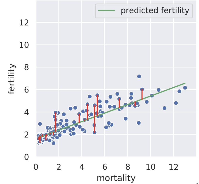
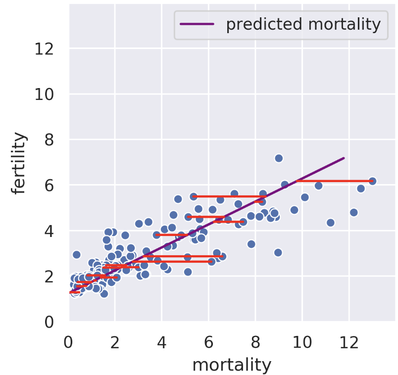
Suppose we know the child mortality rate of a given country. Linear regression tries to predict the fertility rate from the mortality rate; for example, if the mortality is 6, we might guess the fertility is near 4. The regression line tells us the “best” prediction of fertility given all possible mortality values by minimizing the root mean squared error. See the vertical red lines (note that only some are shown).
We can also perform a regression in the reverse direction. That is, given fertility, we try to predict mortality. In this case, we get a different regression line that minimizes the root mean squared length of the horizontal lines.
25.10.2 SVD: Minimizing Perpendicular Error
The rank-1 approximation is close but not the same as the mortality regression line. Instead of minimizing horizontal or vertical error, our rank-1 approximation minimizes the error perpendicular to the subspace onto which we’re projecting. That is, SVD finds the line such that if we project our data onto that line, the error between the projection and our original data is minimized. The similarity of the rank-1 approximation and the fertility was just a coincidence. Looking at adiposity and bicep size from our body measurements dataset, we see the 1D subspace onto which we are projecting is between the two regression lines.
25.10.3 Beyond 1D and 2D
Even in higher dimensions, the idea behind principal components is the same! Suppose we have 30-dimensional data and decide to use the first 5 principal components. Our procedure minimizes the error between the original 30-dimensional data and the projection of that 30-dimensional data onto the “best” 5-dimensional subspace. See CS 189 Note 10 for more details.
25.11 [BONUS] Automatic Factorization
One key fact to remember is that the decomposition is not arbitrary. The rank of a matrix limits how small our inner dimensions can be if we want to perfectly recreate our matrix. The proof for this is out of scope.
Even if we know we have to factorize our matrix using an inner dimension of \(R\), that still leaves a large space of solutions to traverse. What if we have a procedure to automatically factorize a rank \(R\) matrix into an \(R\)-dimensional representation with some transformation matrix?
Imagine a 1000-dimensional dataset: If the rank is only 5, it’s much easier to do EDA after this mystery procedure.
What if we wanted a 2D representation? It’s valuable to compress all of the data that is relevant into as few dimensions as possible in order to plot it efficiently. Some 2D matrices yield better approximations than others. How well can we do?
25.12 [BONUS] Proof of Component Score
The proof defining component score is out of scope for this class, but it is included below for your convenience.
Setup: Consider the design matrix \(X \in \mathbb{R}^{n \times d}\), where the \(j\)-th column (corresponding to the \(j\)-th feature) is \(x_j \in \mathbb{R}^n\) and the element in row \(i\), column \(j\) is \(x_{ij}\). Further, define \(\tilde{X}\) as the centered design matrix. The \(j\)-th column is \(\tilde{x}_j \in \mathbb{R}^n\) and the element in row \(i\), column \(j\) is \(\tilde{x}_{ij} = x_{ij} - \bar{x_j}\), where \(\bar{x_j}\) is the mean of the \(x_j\) column vector from the original \(X\).
Variance: Construct the covariance matrix: \(\frac{1}{n} \tilde{X}^T \tilde{X} \in \mathbb{R}^{d \times d}\). The \(j\)-th element along the diagonal is the variance of the \(j\)-th column of the original design matrix \(X\):
SVD: Suppose singular value decomposition of the centered design matrix \(\tilde{X}\) yields \(\tilde{X} = U S V^T\), where \(U \in \mathbb{R}^{n \times d}\) and \(V \in \mathbb{R}^{d \times d}\) are matrices with orthonormal columns, and \(S \in \mathbb{R}^{d \times d}\) is a diagonal matrix with singular values of \(\tilde{X}\).
\[
\begin{aligned}
\tilde{X}^T \tilde{X} &= (U S V^T )^T (U S V^T) \\
&= V S U^T U S V^T & (S^T = S) \\
&= V S^2 V^T & (U^T U = I) \\
\frac{1}{n} \tilde{X}^T \tilde{X} &= \frac{1}{n} V S V^T =V \left( \frac{1}{n} S \right) V^T \\
\frac{1}{n} \tilde{X}^T \tilde{X} V &= V \left( \frac{1}{n} S \right) V^T V = V \left( \frac{1}{n} S \right) & \text{(right multiply by }V \rightarrow V^T V = I \text{)} \\
V^T \frac{1}{n} \tilde{X}^T \tilde{X} V &= V^T V \left( \frac{1}{n} S \right) = \frac{1}{n} S & \text{(left multiply by }V^T \rightarrow V^T V = I \text{)} \\
\left( \frac{1}{n} \tilde{X}^T \tilde{X} \right)_{jj} &= \frac{1}{n}S_j^2 & \text{(Define }S_j\text{ as the} j\text{-th singular value)} \\
\frac{1}{n} S_j^2 &= \frac{1}{n} \sum_{i=i}^n (x_{ij} - \bar{x_j})^2
\end{aligned}
\]
The last line defines the \(j\)-th component score.