We will introduce the concept of aggregating data – we will familiarize ourselves with GroupBy objects and used them as tools to consolidate and summarize a DataFrame. In this lecture, we will explore working with the different aggregation functions and dive into some advanced .groupby methods to show just how powerful of a resource they can be for understanding our data. We will also introduce other techniques for data aggregation to provide flexibility in how we manipulate our tables.
First, let’s load babynames dataset.
Click to see the code
# This code pulls census data and loads it into a DataFrame
# We won't cover it explicitly in this class, but you are welcome to explore it on your own
import pandas as pd
import numpy as np
import urllib.request
import os.path
import zipfile

data_url = "https://www.ssa.gov/oact/babynames/state/namesbystate.zip"
local_filename = "data/babynamesbystate.zip"
if not os.path.exists(local_filename): # If the data exists don't download again
    with urllib.request.urlopen(data_url) as resp, open(local_filename, 'wb') as f:
        f.write(resp.read())

zf = zipfile.ZipFile(local_filename, 'r')

ca_name = 'STATE.CA.TXT'
field_names = ['State', 'Sex', 'Year', 'Name', 'Count']
with zf.open(ca_name) as fh:
    babynames = pd.read_csv(fh, header=None, names=field_names)

babynames.head()Aggregating Data with .groupby
Up until this point, we have been working with individual rows of DataFrames. As data scientists, we often wish to investigate trends across a larger subset of our data. For example, we may want to compute some summary statistic (the mean, median, sum, etc.) for a group of rows in our DataFrame. To do this, we’ll use pandas GroupBy objects. Our goal is to group together rows that fall under the same category and perform an operation that aggregates across all rows in the category.
Let’s say we wanted to aggregate all rows in babynames for a given year.
babynames.groupby("Year")<pandas.core.groupby.generic.DataFrameGroupBy object at 0x12fc94290>What does this strange output mean? Calling .groupby (documentation) has generated a GroupBy object. You can imagine this as a set of “mini”, grouped sub-DataFrames, where each group/sub-DataFrame contains all of the rows from babynames that correspond to a particular year.
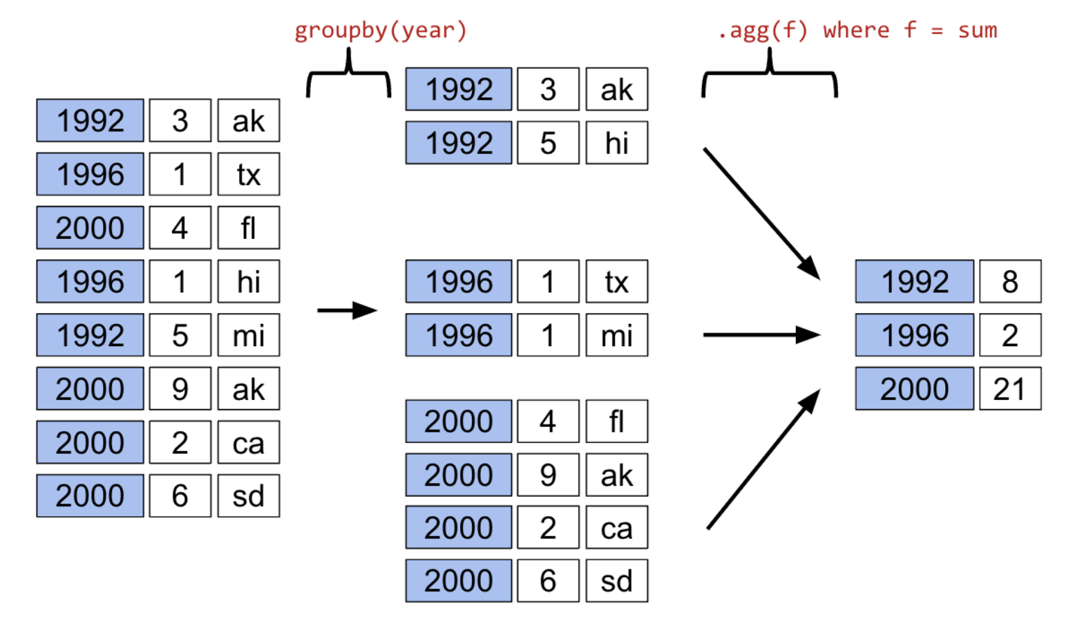
The diagram below shows a simplified view of babynames to help illustrate this idea.
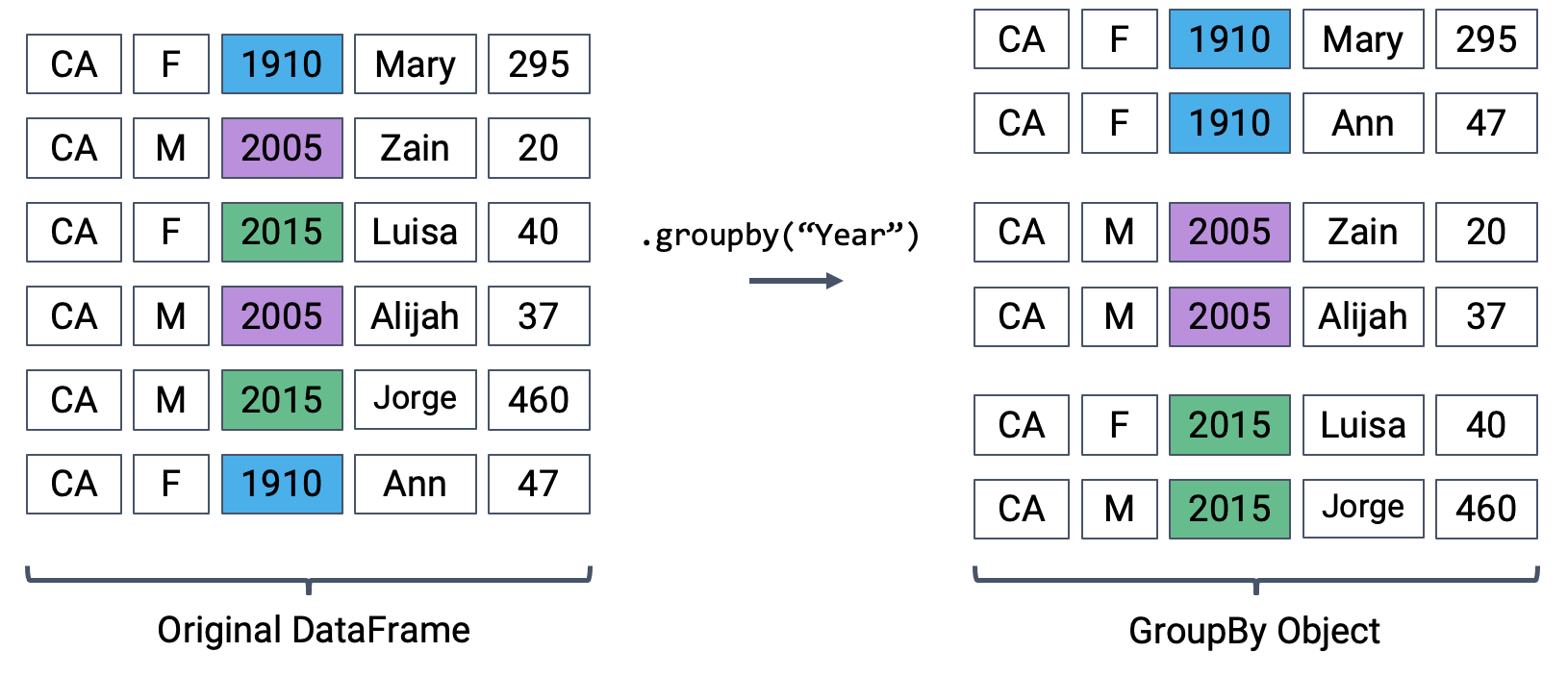
We can’t work with a GroupBy object directly – that is why you saw that strange output earlier rather than a standard view of a DataFrame. To actually manipulate values within these groups/sub-DataFrames, we’ll need to call an aggregation method. This is a method that tells pandas how to aggregate the values within the GroupBy object. Once the aggregation is applied, pandas will return a normal (now grouped) DataFrame.
The first aggregation method we’ll consider is .agg. The .agg method takes in a function as its argument; this function is then applied to each column of a group/sub-DataFrame. We end up with a new DataFrame with one aggregated row per subframe. Let’s see this in action by finding the sum of all counts for each year in babynames – this is equivalent to finding the number of babies born in each year.
babynames[["Year", "Count"]].groupby("Year").agg("sum").head(5)We can relate this back to the diagram we used above. Remember that the diagram uses a simplified version of babynames, which is why we see smaller values for the summed counts.
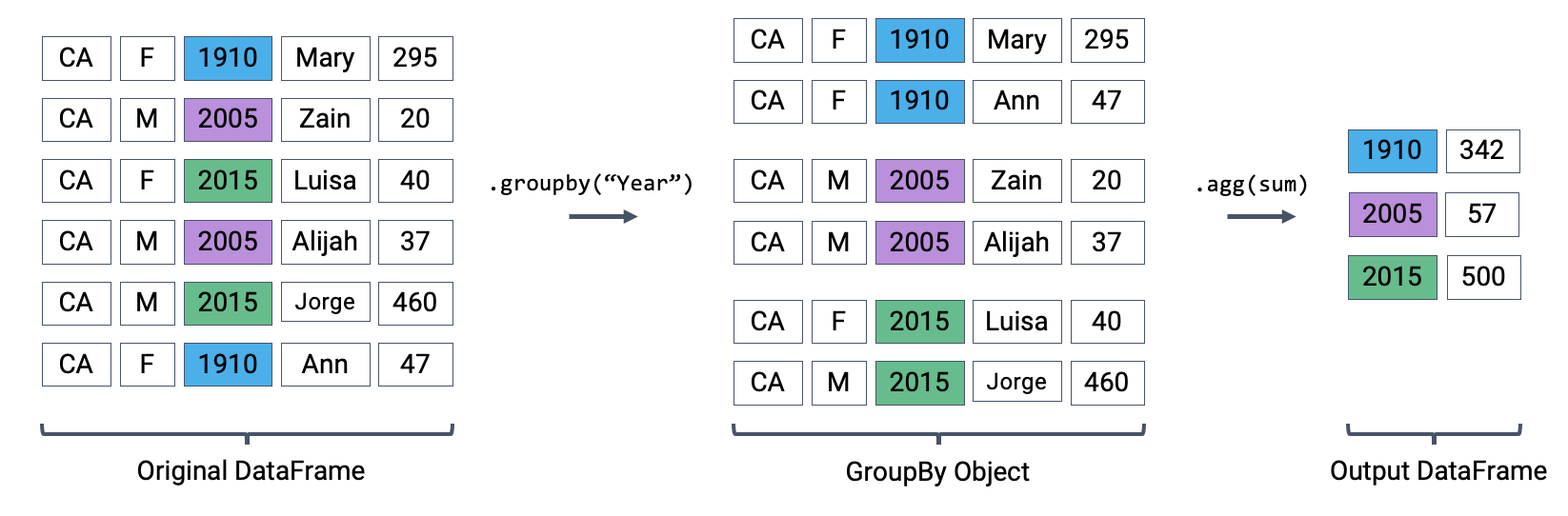
Calling .agg has condensed each subframe (i.e. group/sub-DataFrame) back into a single row. This gives us our final output: a DataFrame that is now indexed by "Year", with a single row for each unique year in the original babynames DataFrame.
There are many different aggregation functions we can use, all of which are useful in different applications.
babynames[["Year", "Count"]].groupby("Year").agg("min").head(5)babynames[["Year", "Count"]].groupby("Year").agg("max").head(5)# Same result, but now we explicitly tell pandas to only consider the "Count" column when summing
babynames.groupby("Year")[["Count"]].agg("sum").head(5)There are many different aggregations that can be applied to the grouped data. The primary requirement is that an aggregation function must:
Take in a
Seriesof data (a single column of the grouped subframe).Return a single value that aggregates this
Series.
Aggregation Functions
Because of this fairly broad requirement, pandas offers many ways of computing an aggregation.
In-built Python operations – such as sum, max, and min – are automatically recognized by pandas.
# What is the minimum count for each name in any year?
babynames.groupby("Name")[["Count"]].agg("min").head()# What is the largest single-year count of each name?
babynames.groupby("Name")[["Count"]].agg("max").head()As mentioned previously, functions from the NumPy library, such as np.mean, np.max, np.min, and np.sum, are also fair game in pandas.
# What is the average count for each name across all years?
babynames.groupby("Name")[["Count"]].agg("mean").head()pandas also offers a number of in-built functions. Functions that are native to pandas can be referenced using their string name within a call to .agg. Some examples include:
.agg("sum").agg("max").agg("min").agg("mean").agg("first").agg("last")
The latter two entries in this list – "first" and "last" – are unique to pandas. They return the first or last entry in a subframe column. Why might this be useful? Consider a case where multiple columns in a group share identical information. To represent this information in the grouped output, we can simply grab the first or last entry, which we know will be identical to all other entries.
Let’s illustrate this with an example. Say we add a new column to babynames that contains the first letter of each name.
# Imagine we had an additional column, "First Letter". We'll explain this code next week
babynames["First Letter"] = babynames["Name"].str[0]

# We construct a simplified DataFrame containing just a subset of columns
babynames_new = babynames[["Name", "First Letter", "Year"]]
babynames_new.head()If we form groups for each name in the dataset, "First Letter" will be the same for all members of the group. This means that if we simply select the first entry for "First Letter" in the group, we’ll represent all data in that group.
We can use a dictionary to apply different aggregation functions to each column during grouping.
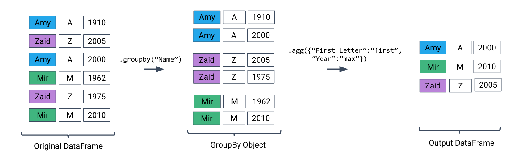
babynames_new.groupby("Name").agg({"First Letter":"first", "Year":"max"}).head()Plotting Birth Counts
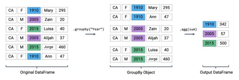
Let’s use .agg to find the total number of babies born in each year. Recall that using .agg with .groupby() follows the format: df.groupby(column_name).agg(aggregation_function). The line of code below gives us the total number of babies born in each year.
Click to see the code
babynames.groupby("Year")[["Count"]].agg(sum).head(5)
# Alternative 1
# babynames.groupby("Year")[["Count"]].sum()
# Alternative 2
# babynames.groupby("Year").sum(numeric_only=True)Here’s an illustration of the process:
Plotting the DataFrame we obtain tells an interesting story.
Click to see the code
import plotly.express as px
puzzle2 = babynames.groupby("Year")[["Count"]].agg("sum")
px.line(puzzle2, y = "Count")A word of warning: we made an enormous assumption when we decided to use this dataset to estimate birth rate. According to this article from the Legislative Analyst’s Office, the true number of babies born in California in 2020 was 421,275. However, our plot shows 362,882 babies —— what happened?
Summary of the .groupby() Function
A groupby operation involves some combination of splitting a DataFrame into grouped subframes, applying a function, and combining the results.
For some arbitrary DataFrame df below, the code df.groupby("year").agg(sum) does the following:
Splits the
DataFrameinto sub-DataFrames with rows belonging to the same year.Applies the
sumfunction to each column of each sub-DataFrame.Combines the results of
suminto a singleDataFrame, indexed byyear.
Revisiting the .agg() Function
.agg() can take in any function that aggregates several values into one summary value. Some commonly-used aggregation functions can even be called directly, without explicit use of .agg(). For example, we can call .mean() on .groupby():
babynames.groupby("Year").mean().head()We can now put this all into practice. Say we want to find the baby name with sex “F” that has fallen in popularity the most in California. To calculate this, we can first create a metric: “Ratio to Peak” (RTP). The RTP is the ratio of babies born with a given name in 2022 to the maximum number of babies born with the name in any year.
Let’s start with calculating this for one baby, “Jennifer”.
# We filter by babies with sex "F" and sort by "Year"
f_babynames = babynames[babynames["Sex"] == "F"]
f_babynames = f_babynames.sort_values(["Year"])

# Determine how many Jennifers were born in CA per year
jenn_counts_series = f_babynames[f_babynames["Name"] == "Jennifer"]["Count"]

# Determine the max number of Jennifers born in a year and the number born in 2022
# to calculate RTP
max_jenn = max(f_babynames[f_babynames["Name"] == "Jennifer"]["Count"])
curr_jenn = f_babynames[f_babynames["Name"] == "Jennifer"]["Count"].iloc[-1]
rtp = curr_jenn / max_jenn
rtp0.018796372629843364By creating a function to calculate RTP and applying it to our DataFrame by using .groupby(), we can easily compute the RTP for all names at once!
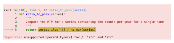
def ratio_to_peak(series):
    return series.iloc[-1] / max(series)

#Using .groupby() to apply the function
rtp_table = f_babynames.groupby("Name")[["Year", "Count"]].agg(ratio_to_peak)
rtp_table.head()In the rows shown above, we can see that every row shown has a Year value of 1.0.
This is the “pandas-ification” of logic you saw in Data 8. Much of the logic you’ve learned in Data 8 will serve you well in Data 100.
Nuisance Columns
Note that you must be careful with which columns you apply the .agg() function to. If we were to apply our function to the table as a whole by doing f_babynames.groupby("Name").agg(ratio_to_peak), executing our .agg() call would result in a TypeError.
We can avoid this issue (and prevent unintentional loss of data) by explicitly selecting column(s) we want to apply our aggregation function to BEFORE calling .agg(),
Renaming Columns After Grouping
By default, .groupby will not rename any aggregated columns. As we can see in the table above, the aggregated column is still named Count even though it now represents the RTP. For better readability, we can rename Count to Count RTP
rtp_table = rtp_table.rename(columns = {"Count": "Count RTP"})
rtp_tableSome Data Science Payoff
By sorting rtp_table, we can see the names whose popularity has decreased the most.
rtp_table = rtp_table.rename(columns = {"Count": "Count RTP"})
rtp_table.sort_values("Count RTP").head()To visualize the above DataFrame, let’s look at the line plot below:
Click to see the code
import plotly.express as px
px.line(f_babynames[f_babynames["Name"] == "Debra"], x = "Year", y = "Count")We can get the list of the top 10 names and then plot popularity with the following code:
top10 = rtp_table.sort_values("Count RTP").head(10).index
px.line(
    f_babynames[f_babynames["Name"].isin(top10)],
    x = "Year",
    y = "Count",
    color = "Name"
)As a quick exercise, consider what code would compute the total number of babies with each name.
Click to see the code
babynames.groupby("Name")[["Count"]].agg("sum").head()
# alternative solution:
# babynames.groupby("Name")[["Count"]].sum().groupby(), Continued
We’ll work with the elections DataFrame again.
Click to see the code
import pandas as pd
import numpy as np

elections = pd.read_csv("data/elections.csv")
elections.head(5)Raw GroupBy Objects
The result of groupby applied to a DataFrame is a DataFrameGroupBy object, not a DataFrame.
grouped_by_year = elections.groupby("Year")
type(grouped_by_year)pandas.core.groupby.generic.DataFrameGroupByThere are several ways to look into DataFrameGroupBy objects:
grouped_by_party = elections.groupby("Party")
grouped_by_party.groups
{'American': [22, 126], 'American Independent': [115, 119, 124], 'Anti-Masonic': [6], 'Anti-Monopoly': [38], 'Citizens': [127], 'Communist': [89], 'Constitution': [160, 164, 172], 'Constitutional Union': [24], 'Democratic': [2, 4, 8, 10, 13, 14, 17, 20, 28, 29, 34, 37, 39, 45, 47, 52, 55, 57, 64, 70, 74, 77, 81, 83, 86, 91, 94, 97, 100, 105, 108, 111, 114, 116, 118, 123, 129, 134, 137, 140, 144, 151, 158, 162, 168, 176, 178, 183], 'Democratic-Republican': [0, 1], 'Dixiecrat': [103], 'Farmer–Labor': [78], 'Free Soil': [15, 18], 'Green': [149, 155, 156, 165, 170, 177, 181, 184], 'Greenback': [35], 'Independent': [121, 130, 143, 161, 167, 174, 185], 'Liberal Republican': [31], 'Libertarian': [125, 128, 132, 138, 139, 146, 153, 159, 163, 169, 175, 180], 'Libertarian Party': [186], 'National Democratic': [50], 'National Republican': [3, 5], 'National Union': [27], 'Natural Law': [148], 'New Alliance': [136], 'Northern Democratic': [26], 'Populist': [48, 61, 141], 'Progressive': [68, 82, 101, 107], 'Prohibition': [41, 44, 49, 51, 54, 59, 63, 67, 73, 75, 99], 'Reform': [150, 154], 'Republican': [21, 23, 30, 32, 33, 36, 40, 43, 46, 53, 56, 60, 65, 69, 72, 79, 80, 84, 87, 90, 96, 98, 104, 106, 109, 112, 113, 117, 120, 122, 131, 133, 135, 142, 145, 152, 157, 166, 171, 173, 179, 182], 'Socialist': [58, 62, 66, 71, 76, 85, 88, 92, 95, 102], 'Southern Democratic': [25], 'States' Rights': [110], 'Taxpayers': [147], 'Union': [93], 'Union Labor': [42], 'Whig': [7, 9, 11, 12, 16, 19]}grouped_by_party.get_group("Socialist")Other GroupBy Methods
There are many aggregation methods we can use with .agg. Some useful options are:
.mean()documentation: creates a newDataFramewith the mean value of each group.sum()documentation: creates a newDataFramewith the sum of each group.max()documentation and.min()documentation: creates a newDataFramewith the maximum/minimum value of each group.first()documentation and.last()documentation: creates a newDataFramewith the first/last row in each group.head(n)documentation and.tail(n)documentation: creates a newDataFramewith the first/lastnrows in each group.size()documentation: creates a newSerieswith the number of entries in each group.count()documentation: creates a newDataFramewith the number of entries, excluding missing values.
Let’s illustrate some examples by creating a DataFrame called df.
df = pd.DataFrame({'letter':['A','A','B','C','C','C'],
                   'num':[1,2,3,4,np.nan,4],
                   'state':[np.nan, 'tx', 'fl', 'hi', np.nan, 'ak']})
dfNote the slight difference between .size() and .count(): while .size() returns a Series and counts the number of entries including the missing values, .count() returns a DataFrame and counts the number of entries in each column excluding missing values.
df.groupby("letter").size()letter
A 2
B 1
C 3
dtype: int64df.groupby("letter").count()You might recall that the value_counts() function in the previous note does something similar. It turns out value_counts() and groupby.size() are the same, except value_counts() sorts the resulting Series in descending order automatically.
df["letter"].value_counts()letter
C 3
A 2
B 1
Name: count, dtype: int64These (and other) aggregation functions are so common that pandas allows for writing shorthand. Instead of explicitly stating the use of .agg, we can call the function directly on the GroupBy object.
For example, the following are equivalent:
elections.groupby("Candidate").agg(mean)elections.groupby("Candidate").mean()
There are many other methods that pandas supports. You can check them out on the pandas documentation.
Filtering by Group
Another common use for GroupBy objects is to filter data by group.
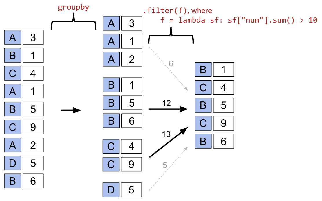
groupby.filter takes an argument func, where func is a function that:
Takes a
DataFrameobject as inputReturns a single
TrueorFalse.
groupby.filter applies func to each group/sub-DataFrame:
If
funcreturnsTruefor a group, then all rows belonging to the group are preserved.If
funcreturnsFalsefor a group, then all rows belonging to that group are filtered out.
In other words, sub-DataFrames that correspond to True are returned in the final result, whereas those with a False value are not. Importantly, groupby.filter is different from groupby.agg in that an entire sub-DataFrame is returned in the final DataFrame, not just a single row. As a result, groupby.filter preserves the original indices and the column we grouped on does NOT become the index!
sf refers to subframe or sub-DataFrame which are the “mini”, grouped sub-DataFrames.
To illustrate how this happens, let’s go back to the elections dataset. Say we want to identify “tight” election years – that is, we want to find all rows that correspond to election years where all candidates in that year won a similar portion of the total vote. Specifically, let’s find all rows corresponding to a year where no candidate won more than 45% of the total vote.
In other words, we want to:
Find the years where the maximum
%in that year is less than 45%Return all
DataFramerows that correspond to these years
For each year, we need to find the maximum % among all rows for that year. If this maximum % is lower than 45%, we will tell pandas to keep all rows corresponding to that year.
elections.groupby("Year").filter(lambda sf: sf["%"].max() < 45).head(9)What’s going on here? In this example, we’ve defined our filtering function, func, to be lambda sf: sf["%"].max() < 45. This filtering function will find the maximum "%" value among all entries in the grouped sub-DataFrame, which we call sf. If the maximum value is less than 45, then the filter function will return True and all rows in that grouped sub-DataFrame will appear in the final output DataFrame.
Examine the DataFrame above. Notice how, in this preview of the first 9 rows, all entries from the years 1860 and 1912 appear. This means that in 1860 and 1912, no candidate in that year won more than 45% of the total vote.
You may ask: how is the groupby.filter procedure different to the boolean filtering we’ve seen previously? Boolean filtering considers individual rows when applying a boolean condition. For example, the code elections[elections["%"] < 45] will check the "%" value of every single row in elections; if it is less than 45, then that row will be kept in the output. groupby.filter, in contrast, applies a boolean condition across all rows in a group. If not all rows in that group satisfy the condition specified by the filter, the entire group will be discarded in the output.
Aggregation with lambda Functions
What if we wish to aggregate our DataFrame using a non-standard function – for example, a function of our own design? We can do so by combining .agg with lambda expressions.
Let’s first consider a puzzle to jog our memory. We will attempt to find the Candidate from each Party with the highest % of votes.
A naive approach may be to group by the Party column and aggregate by the maximum.
elections.groupby("Party").agg("max").head(10)This approach is clearly wrong – the DataFrame claims that Woodrow Wilson won the presidency in 2024.
Why is this happening? Here, the max aggregation function is taken over every column independently. Among Democrats, max is computing:
The most recent
Yeara Democratic candidate ran for president (2024)The
Candidatewith the alphabetically “largest” name (“Woodrow Wilson”)The
Resultwith the alphabetically “largest” outcome (“win”)
Instead, let’s try a different approach. We will:
Sort the
DataFrameso that rows are in descending order of%Group by
Partyand select the first row of each sub-DataFrame
While it may seem unintuitive, sorting elections by descending order of % is extremely helpful. If we then group by Party, the first row of each GroupBy object will contain information about the Candidate with the highest voter %.
elections_sorted_by_percent = elections.sort_values("%", ascending=False)
elections_sorted_by_percent.head(5)elections_sorted_by_percent.groupby("Party").agg(lambda x : x.iloc[0]).head(10)
# Equivalent to the below code
# elections_sorted_by_percent.groupby("Party").agg('first').head(10)Here’s an illustration of the process:
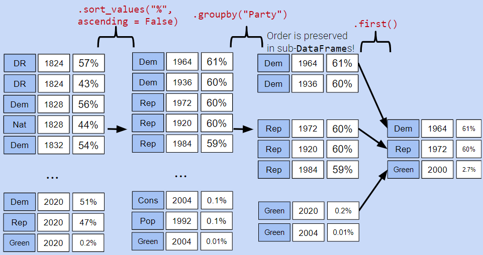
Notice how our code correctly determines that Lyndon Johnson from the Democratic Party has the highest voter %.
More generally, lambda functions are used to design custom aggregation functions that aren’t pre-defined by Python. The input parameter x to the lambda function is a GroupBy object. Therefore, it should make sense why lambda x : x.iloc[0] selects the first row in each groupby object.
In fact, there’s a few different ways to approach this problem. Each approach has different tradeoffs in terms of readability, performance, memory consumption, complexity, etc. We’ve given a few examples below.
Note: Understanding these alternative solutions is not required. They are given to demonstrate the vast number of problem-solving approaches in pandas.
# Using the idxmax function
best_per_party = elections.loc[elections.groupby('Party')['%'].idxmax()]
best_per_party.head(5)# Using the .drop_duplicates function
best_per_party2 = elections.sort_values('%').drop_duplicates(['Party'], keep='last')
best_per_party2.head(5)Aggregating Data with Pivot Tables
We know now that .groupby gives us the ability to group and aggregate data across our DataFrame. The examples above formed groups using just one column in the DataFrame. It’s possible to group by multiple columns at once by passing in a list of column names to .groupby.
Let’s consider the babynames dataset again. In this problem, we will find the total number of baby names associated with each sex for each year. To do this, we’ll group by both the "Year" and "Sex" columns.
babynames.head()# Find the total number of baby names associated with each sex for each
# year in the data
babynames.groupby(["Year", "Sex"])[["Count"]].agg("sum").head(6)Notice that both "Year" and "Sex" serve as the index of the DataFrame (they are both rendered in bold). We’ve created a multi-index DataFrame where two different index values, the year and sex, are used to uniquely identify each row.
This isn’t the most intuitive way of representing this data – and, because multi-indexed DataFrames have multiple dimensions in their index, they can often be difficult to use.
Another strategy to aggregate across two columns is to create a pivot table. You saw these back in Data 8. One set of values is used to create the index of the pivot table; another set is used to define the column names. The values contained in each cell of the table correspond to the aggregated data for each index-column pair.
Here’s an illustration of the process:
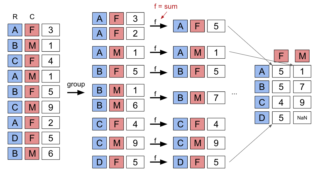
The best way to understand pivot tables is to see one in action. Let’s return to our original goal of summing the total number of names associated with each combination of year and sex. We’ll call the pandas .pivot_table documentation method to create a new table.
# The `pivot_table` method is used to generate a Pandas pivot table
import numpy as np
babynames.pivot_table(
    index = "Year",
    columns = "Sex",
    values = "Count",
    aggfunc = "sum",
).head(5)Looks a lot better! Now, our DataFrame is structured with clear index-column combinations. Each entry in the pivot table represents the summed count of names for a given combination of "Year" and "Sex".
Let’s take a closer look at the code implemented above.
index = "Year"specifies the column name in the originalDataFramethat should be used as the index of the pivot tablecolumns = "Sex"specifies the column name in the originalDataFramethat should be used to generate the columns of the pivot tablevalues = "Count"indicates what values from the originalDataFrameshould be used to populate the entry for each index-column combinationaggfunc = np.sumtellspandaswhat function to use when aggregating the data specified byvalues. Here, we are summing the name counts for each pair of"Year"and"Sex"
We can even include multiple values in the index or columns of our pivot tables.
babynames_pivot = babynames.pivot_table(
    index="Year",     # the rows (turned into index)
    columns="Sex",    # the column values
    values=["Count", "Name"],
    aggfunc="max",      # group operation
)
babynames_pivot.head(6)Note that each row provides the number of girls and number of boys having that year’s most common name, and also lists the alphabetically largest girl name and boy name. The counts for number of girls/boys in the resulting DataFrame do not correspond to the names listed. For example, in 1910, the most popular girl name is given to 295 girls, but that name was likely not Yvonne.
Joining Tables
When working on data science projects, we’re unlikely to have absolutely all the data we want contained in a single DataFrame – a real-world data scientist needs to grapple with data coming from multiple sources. If we have access to multiple datasets with related information, we can join two or more tables into a single DataFrame.
To put this into practice, we’ll revisit the elections dataset.
elections.head(5)Say we want to understand the popularity of the names of each presidential candidate in 2022. To do this, we’ll need the combined data of babynames and elections.
We’ll start by creating a new column containing the first name of each presidential candidate. This will help us join each name in elections to the corresponding name data in babynames.
# This `str` operation splits each candidate's full name at each
# blank space, then takes just the candidate's first name
elections["First Name"] = elections["Candidate"].str.split().str[0]
elections.head(5)# Here, we'll only consider `babynames` data from 2022
babynames_2022 = babynames[babynames["Year"]==2022]
babynames_2022.head()Now, we’re ready to join the two tables. pd.merge (documentation) is the pandas method used to join DataFrames together.
merged = pd.merge(left = elections, right = babynames_2022, \
                  left_on = "First Name", right_on = "Name")
merged.head()
# Notice that pandas automatically specifies `Year_x` and `Year_y`
# when both merged DataFrames have the same column name to avoid confusion

# Second option
# merged = elections.merge(right = babynames_2022, \
# left_on = "First Name", right_on = "Name")Let’s take a closer look at the parameters:
leftandrightparameters are used to specify theDataFrames to be joined.left_onandright_onparameters are assigned to the string names of the columns to be used when performing the join. These twoonparameters tellpandaswhat values should act as pairing keys to determine which rows to merge across theDataFrames. We’ll talk more about this idea of a pairing key next lecture.
Parting Note
Congratulations! We finally tackled pandas. Don’t worry if you are still not feeling very comfortable with it—you will have plenty of chances to practice over the next few weeks.
Next, we will get our hands dirty with some real-world datasets and use our pandas knowledge to conduct some exploratory data analysis.