In the past few lectures, we’ve learned that pandas is a toolkit to restructure, modify, and explore a dataset. What we haven’t yet touched on is how to make these data transformation decisions. When we receive a new set of data from the “real world,” how do we know what processing we should do to convert this data into a usable form?
Data cleaning, also called data wrangling, is the process of transforming raw data to facilitate subsequent analysis. It is often used to address issues like:
Unclear structure or formatting
Missing or corrupted values
Unit conversions
...and so on
Exploratory Data Analysis (EDA) is the process of understanding a new dataset. It is an open-ended, informal analysis that involves familiarizing ourselves with the variables present in the data, discovering potential hypotheses, and identifying possible issues with the data. This last point can often motivate further data cleaning to address any problems with the dataset’s format; because of this, EDA and data cleaning are often thought of as an “infinite loop,” with each process driving the other.
In this lecture, we will consider the key properties of data to consider when performing data cleaning and EDA. In doing so, we’ll develop a “checklist” of sorts for you to consider when approaching a new dataset. Throughout this process, we’ll build a deeper understanding of this early (but very important!) stage of the data science lifecycle.
Structure
We often prefer rectangular data for data analysis. Rectangular structures are easy to manipulate and analyze. A key element of data cleaning is about transforming data to be more rectangular.
There are two kinds of rectangular data: tables and matrices. Tables have named columns with different data types and are manipulated using data transformation languages. Matrices contain numeric data of the same type and are manipulated using linear algebra.
File Formats
There are many file types for storing structured data: TSV, JSON, XML, ASCII, SAS, etc. We’ll only cover CSV, TSV, and JSON in lecture, but you’ll likely encounter other formats as you work with different datasets. Reading documentation is your best bet for understanding how to process the multitude of different file types.
CSV
CSVs, which stand for Comma-Separated Values, are a common tabular data format.
In the past two pandas lectures, we briefly touched on the idea of file format: the way data is encoded in a file for storage. Specifically, our elections and babynames datasets were stored and loaded as CSVs:
pd.read_csv("data/elections.csv").head(5)To better understand the properties of a CSV, let’s take a look at the first few rows of the raw data file to see what it looks like before being loaded into a DataFrame. We’ll use the repr() function to return the raw string with its special characters:
with open("data/elections.csv", "r") as table:
    i = 0
    for row in table:
        print(repr(row))
        i += 1
        if i > 3:
            break
'Year,Candidate,Party,Popular vote,Result,%\n'
'1824,Andrew Jackson,Democratic-Republican,151271,loss,57.21012204\n'
'1824,John Quincy Adams,Democratic-Republican,113142,win,42.78987796\n'
'1828,Andrew Jackson,Democratic,642806,win,56.20392707\n'
Each row, or record, in the data is delimited by a newline \n. Each column, or field, in the data is delimited by a comma , (hence, comma-separated!).
TSV
Another common file type is TSV (Tab-Separated Values). In a TSV, records are still delimited by a newline \n, while fields are delimited by \t tab character.
Let’s check out the first few rows of the raw TSV file. Again, we’ll use the repr() function so that print shows the special characters.
with open("data/elections.txt", "r") as table:
    i = 0
    for row in table:
        print(repr(row))
        i += 1
        if i > 3:
            break
'\ufeffYear\tCandidate\tParty\tPopular vote\tResult\t%\n'
'1824\tAndrew Jackson\tDemocratic-Republican\t151271\tloss\t57.21012204\n'
'1824\tJohn Quincy Adams\tDemocratic-Republican\t113142\twin\t42.78987796\n'
'1828\tAndrew Jackson\tDemocratic\t642806\twin\t56.20392707\n'
TSVs can be loaded into pandas using pd.read_csv. We’ll need to specify the delimiter with parameter sep='\t' (documentation).
pd.read_csv("data/elections.txt", sep='\t').head(3)An issue with CSVs and TSVs comes up whenever there are commas or tabs within the records. How does pandas differentiate between a comma delimiter vs. a comma within the field itself, for example 8,900? To remedy this, check out the quotechar parameter.
JSON
JSON (JavaScript Object Notation) files behave similarly to Python dictionaries. A raw JSON is shown below.
with open("data/elections.json", "r") as table:
    i = 0
    for row in table:
        print(row)
        i += 1
        if i > 8:
            break
[
{
"Year": 1824,
"Candidate": "Andrew Jackson",
"Party": "Democratic-Republican",
"Popular vote": 151271,
"Result": "loss",
"%": 57.21012204
},
JSON files can be loaded into pandas using pd.read_json.
pd.read_json('data/elections.json').head(3)EDA with JSON: United States Congress Data
The congress.gov API (Application Programming Interface) provides data about the activities and members of the United States Congress (i.e., the House of Representatives and the Senate).
To get a JSON file containing information about the current members of Congress from California, you could use the following API call:
https://api.congress.gov/v3/member/CA?api_key=[INSERT_KEY]&limit=250&format=json¤tMember=TrueYou can instantly sign up for a congress.gov API key here. Once you have your key, replace
[INSERT_KEY]above with your key, and enter the API call as a URL in your browser. What happens?Once the JSON from the API call is visible in your browser, you can click
File-->Save Page Asto save the JSON file to your coputer.Coarsely, API keys are used to track how much a given user engages with the API. There might be limits to the number of API calls (e.g., congress.gov API limits to 5,000 calls per hour), or a cost for API calls (e.g., using the OpenAI API for programmatically using ChatGPT).
After following these steps, we save this JSON file as data/ca-congress-members.json.
File Contents
Let’s examine this file using Python. We can programmatically view the first couple lines of the file using the same functions we used with CSVs:
congress_file = "data/ca-congress-members.json"

# Inspect the first five lines of the file
with open(congress_file, "r") as f:
    for i, row in enumerate(f):
        print(row)
        if i >= 4: break
{
"members": [
{
"bioguideId": "T000491",
"depiction": {
EDA: Digging into JSON with Python
JSON data closely matches the internal Python object model.
In the following cell, we import the entire JSON datafile into a Python dictionary using the
jsonpackage.
import json

# Import the JSON file into Python as a dictionary
with open(congress_file, "rb") as f:
    congress_json = json.load(f)

type(congress_json)dictThe congress_json variable is a dictionary encoding the data in the JSON file.
Below, we access the first element of the members element of the congress_json dictionary.
This first element is also a dictionary (and there are more dictionaries inside of it!)
# Grab the list corresponding to the `members` key in the JSON dictionary,
# and then grab the first element of this list.
# In a moment, we'll see how we knew to use the key `members`, and that
# the resulting object is a list.
congress_json['members'][0]
{'bioguideId': 'T000491',
'depiction': {'attribution': 'Image courtesy of the Member',
'imageUrl': 'https://www.congress.gov/img/member/6774606d0b34857ecc9091a9_200.jpg'},
'district': 45,
'name': 'Tran, Derek',
'partyName': 'Democratic',
'state': 'California',
'terms': {'item': [{'chamber': 'House of Representatives',
'startYear': 2025}]},
'updateDate': '2025-01-21T18:00:52Z',
'url': 'https://api.congress.gov/v3/member/T000491?format=json'}How should we probe a nested dictionary like congress_json?
We can start by identifying the top-level keys of the dictionary:
# Grab the top-level keys of the JSON dictionary
congress_json.keys()
dict_keys(['members', 'pagination', 'request'])Looks like we have three top-level keys: members, pagination, and request.
You’ll often see a top-level
metakey in JSON files. This does not refer to Meta (formerly Facebook). Instead, it typically refers to metadata (data about the data). Metadata are often maintained alongside the data.
Let’s check the type of the members element:
type(congress_json['members'])listLooks like a list! What are the first two elements?
congress_json['members'][:2][{'bioguideId': 'T000491',
'depiction': {'attribution': 'Image courtesy of the Member',
'imageUrl': 'https://www.congress.gov/img/member/6774606d0b34857ecc9091a9_200.jpg'},
'district': 45,
'name': 'Tran, Derek',
'partyName': 'Democratic',
'state': 'California',
'terms': {'item': [{'chamber': 'House of Representatives',
'startYear': 2025}]},
'updateDate': '2025-01-21T18:00:52Z',
'url': 'https://api.congress.gov/v3/member/T000491?format=json'},
{'bioguideId': 'M001241',
'depiction': {'attribution': 'Image courtesy of the Member',
'imageUrl': 'https://www.congress.gov/img/member/67744ed90b34857ecc909155_200.jpg'},
'district': 47,
'name': 'Min, Dave',
'partyName': 'Democratic',
'state': 'California',
'terms': {'item': [{'chamber': 'House of Representatives',
'startYear': 2025}]},
'updateDate': '2025-01-21T18:00:52Z',
'url': 'https://api.congress.gov/v3/member/M001241?format=json'}]More dictionaries! You can repeat the process above to traverse the nested dictionary.
You’ll notice that each record of congress_json['members'] looks like it could be a column of a DataFrame.
The keys look a lot like column names, and the values could be the entries in each row.
But, the two other elements of congress_json don’t have the same structure as congress_json['members'].
So, they probably don’t belong in a DataFrame containing the members of Congress from CA.
We’ll see the implications of this inconsistency in the next section.
print(congress_json['pagination'])
print(congress_json['request'])
{'count': 54}
{'contentType': 'application/json', 'format': 'json'}
JSON with pandas
pandas has a built in function called pd.read_json for reading in JSON files. In order to read in this JSON file, you might want to try something like the code in the cell below. However, if we tried to run this code, it would error.
# This line intentionally produces an error
pd.read_json(congress_file)
---------------------------------------------------------------------------
ValueError Traceback (most recent call last)
Cell In[15], line 2
1 # This line intentionally produces an error
----> 2 pd.read_json(congress_file)
File c:\Users\kaiwe\anaconda3\envs\data100\Lib\site-packages\pandas\io\json\_json.py:815, in read_json(path_or_buf, orient, typ, dtype, convert_axes, convert_dates, keep_default_dates, precise_float, date_unit, encoding, encoding_errors, lines, chunksize, compression, nrows, storage_options, dtype_backend, engine)
813 return json_reader
814 else:
--> 815 return json_reader.read()
File c:\Users\kaiwe\anaconda3\envs\data100\Lib\site-packages\pandas\io\json\_json.py:1014, in JsonReader.read(self)
1012 obj = self._get_object_parser(self._combine_lines(data_lines))
1013 else:
-> 1014 obj = self._get_object_parser(self.data)
1015 if self.dtype_backend is not lib.no_default:
1016 return obj.convert_dtypes(
1017 infer_objects=False, dtype_backend=self.dtype_backend
1018 )
File c:\Users\kaiwe\anaconda3\envs\data100\Lib\site-packages\pandas\io\json\_json.py:1040, in JsonReader._get_object_parser(self, json)
1038 obj = None
1039 if typ == "frame":
-> 1040 obj = FrameParser(json, **kwargs).parse()
1042 if typ == "series" or obj is None:
1043 if not isinstance(dtype, bool):
File c:\Users\kaiwe\anaconda3\envs\data100\Lib\site-packages\pandas\io\json\_json.py:1176, in Parser.parse(self)
1174 @final
1175 def parse(self):
-> 1176 self._parse()
1178 if self.obj is None:
1179 return None
File c:\Users\kaiwe\anaconda3\envs\data100\Lib\site-packages\pandas\io\json\_json.py:1391, in FrameParser._parse(self)
1388 orient = self.orient
1390 if orient == "columns":
-> 1391 self.obj = DataFrame(
1392 ujson_loads(json, precise_float=self.precise_float), dtype=None
1393 )
1394 elif orient == "split":
1395 decoded = {
1396 str(k): v
1397 for k, v in ujson_loads(json, precise_float=self.precise_float).items()
1398 }
File c:\Users\kaiwe\anaconda3\envs\data100\Lib\site-packages\pandas\core\frame.py:778, in DataFrame.__init__(self, data, index, columns, dtype, copy)
772 mgr = self._init_mgr(
773 data, axes={"index": index, "columns": columns}, dtype=dtype, copy=copy
774 )
776 elif isinstance(data, dict):
777 # GH#38939 de facto copy defaults to False only in non-dict cases
--> 778 mgr = dict_to_mgr(data, index, columns, dtype=dtype, copy=copy, typ=manager)
779 elif isinstance(data, ma.MaskedArray):
780 from numpy.ma import mrecords
File c:\Users\kaiwe\anaconda3\envs\data100\Lib\site-packages\pandas\core\internals\construction.py:503, in dict_to_mgr(data, index, columns, dtype, typ, copy)
499 else:
500 # dtype check to exclude e.g. range objects, scalars
501 arrays = [x.copy() if hasattr(x, "dtype") else x for x in arrays]
--> 503 return arrays_to_mgr(arrays, columns, index, dtype=dtype, typ=typ, consolidate=copy)
File c:\Users\kaiwe\anaconda3\envs\data100\Lib\site-packages\pandas\core\internals\construction.py:114, in arrays_to_mgr(arrays, columns, index, dtype, verify_integrity, typ, consolidate)
111 if verify_integrity:
112 # figure out the index, if necessary
113 if index is None:
--> 114 index = _extract_index(arrays)
115 else:
116 index = ensure_index(index)
File c:\Users\kaiwe\anaconda3\envs\data100\Lib\site-packages\pandas\core\internals\construction.py:680, in _extract_index(data)
677 raise ValueError("All arrays must be of the same length")
679 if have_dicts:
--> 680 raise ValueError(
681 "Mixing dicts with non-Series may lead to ambiguous ordering."
682 )
684 if have_series:
685 if lengths[0] != len(index):
ValueError: Mixing dicts with non-Series may lead to ambiguous ordering.The code above tries to import the entire JSON file located at
congress_file(congress_json), includingcongress_json['pagination']andcongress_json['request'].We only want to make a DataFrame out of
congress_json['members'].
Instead, let’s try converting the members element of congress_json to a DataFrame by using pd.DataFrame:
# Convert dictionary to DataFrame
congress_df = pd.DataFrame(congress_json['members'])
congress_df.head()We’ve successfully begun to rectangularize our JSON data!
Other Data Formats
So far, we’ve looked at text data that comes in a quite nice format. Although some data cleaning might be necessary, it has still had all of the components of a rectangular dataset. However, not all data comes like this, and there are also different kinds of data we can use. Some examples include:
Image Data: Used for medical diagnosis
Audio Data: Used for speech recognition, sentiment analysis
Video Data: Used for object tracking, facial recognition
Text: Used for LLMs, document review
Even though this may not look tabular at first, all of these formats can be represented in tabular/matrix form! So by learning how to work with tabular data, you are well equipped to deal with other kinds of data as well.
Variable Types
Variables are columns. A variable is a measurement of a particular concept. Variables have two common properties: data type/storage type and variable type/feature type. The data type of a variable indicates how each variable value is stored in memory (integer, floating point, boolean, etc.) and affects which pandas functions are used. The variable type is a conceptualized measurement of information (and therefore indicates what values a variable can take on). Variable type is identified through expert knowledge, exploring the data itself, or consulting the data codebook. The variable type affects how one visualizes and inteprets the data. In this class, “variable types” are conceptual.
After loading data into a file, it’s a good idea to take the time to understand what pieces of information are encoded in the dataset. In particular, we want to identify what variable types are present in our data. Broadly speaking, we can categorize variables into one of two overarching types.
Quantitative variables describe some numeric quantity or amount. Some examples include weights, GPA, CO2 concentrations, someone’s age, or the number of siblings they have.
Qualitative variables, also known as categorical variables, describe data that isn’t measuring some quantity or amount. The sub-categories of categorical data are:
Ordinal qualitative variables: categories with ordered levels. Specifically, ordinal variables are those where the difference between levels has no consistent, quantifiable meaning. Some examples include levels of education (high school, undergrad, grad, etc.), income bracket (low, medium, high), or Yelp rating.
Nominal qualitative variables: categories with no specific order. For example, someone’s political affiliation or Cal ID number.
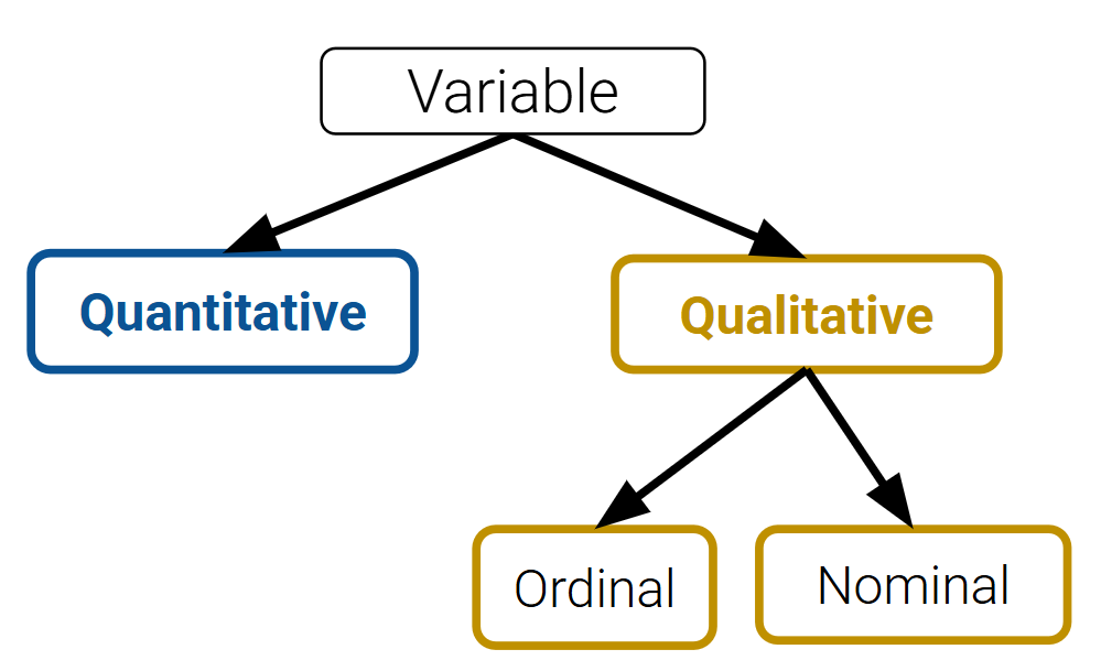
Note that many variables don’t sit neatly in just one of these categories. Qualitative variables could have numeric levels, and conversely, quantitative variables could be stored as strings.
Granularity and Temporality
After understanding the structure of the dataset, the next task is to determine what exactly the data represents. We’ll do so by considering the data’s granularity and temporality.
Granularity
The granularity of a dataset is what a single row represents. You can also think of it as the level of detail included in the data. To determine the data’s granularity, ask: what does each row in the dataset represent? Fine-grained data contains a high level of detail, with a single row representing a small individual unit. For example, each record may represent one person. Coarse-grained data is encoded such that a single row represents a large individual unit – for example, each record may represent a group of people.
Temporality
The temporality of a dataset describes the periodicity over which the data was collected as well as when the data was most recently collected or updated.
Time and date fields of a dataset could represent a few things:
when the “event” happened
when the data was collected, or when it was entered into the system
when the data was copied into the database
To fully understand the temporality of the data, it also may be necessary to standardize time zones or inspect recurring time-based trends in the data (do patterns recur in 24-hour periods? Over the course of a month? Seasonally?). The convention for standardizing time is the Coordinated Universal Time (UTC), an international time standard measured at 0 degrees latitude that stays consistent throughout the year (no daylight savings). We can represent Berkeley’s time zone, Pacific Standard Time (PST), as UTC-7 (with daylight savings).
Temporality with pandas’ dt accessors
Let’s briefly look at how we can use pandas’ dt accessors to work with dates/times in a dataset using the dataset you’ll see in Lab 3: the Berkeley PD Calls for Service dataset.
Click to see the code
calls = pd.read_csv("data/Berkeley_PD_-_Calls_for_Service.csv")
calls.head()Looks like there are three columns with dates/times: EVENTDT, EVENTTM, and InDbDate.
Most likely, EVENTDT stands for the date when the event took place, EVENTTM stands for the time of day the event took place (in 24-hr format), and InDbDate is the date this call is recorded onto the database.
If we check the data type of these columns, we will see they are stored as strings. We can convert them to datetime objects using pandas to_datetime function.
calls["EVENTDT"] = pd.to_datetime(calls["EVENTDT"])
calls.head()Now, we can use the dt accessor on this column.
We can get the month:
calls["EVENTDT"].dt.month.head()Which day of the week the date is on:
calls["EVENTDT"].dt.dayofweek.head()Check the minimum values to see if there are any suspicious-looking, 70s dates:
calls.sort_values("EVENTDT").head()Doesn’t look like it! We are good!
We can also do many things with the dt accessor like switching time zones and converting time back to UNIX/POSIX time. Check out the documentation on .dt accessor and time series/date functionality.
Faithfulness
At this stage in our data cleaning and EDA workflow, we’ve achieved quite a lot: we’ve identified how our data is structured, come to terms with what information it encodes, and gained insight as to how it was generated. Throughout this process, we should always recall the original intent of our work in Data Science – to use data to better understand and model the real world. To achieve this goal, we need to ensure that the data we use is faithful to reality; that is, that our data accurately captures the “real world.”
Data used in research or industry is often “messy” – there may be errors or inaccuracies that impact the faithfulness of the dataset. Signs that data may not be faithful include:
Unrealistic or “incorrect” values, such as negative counts, locations that don’t exist, or dates set in the future
Violations of obvious dependencies, like an age that does not match a birthday
Clear signs that data was entered by hand, which can lead to spelling errors or fields that are incorrectly shifted
Signs of data falsification, such as fake email addresses or repeated use of the same names
Duplicated records or fields containing the same information
Truncated data, e.g. Microsoft Excel would limit the number of rows to 655536 and the number of columns to 255
We often solve some of these more common issues in the following ways:
Spelling errors: apply corrections or drop records that aren’t in a dictionary
Time zone inconsistencies: convert to a common time zone (e.g. UTC)
Duplicated records or fields: identify and eliminate duplicates (using primary keys)
Unspecified or inconsistent units: infer the units and check that values are in reasonable ranges in the data
Missing Values
Another common issue encountered with real-world datasets is that of missing data. One strategy to resolve this is to simply drop any records with missing values from the dataset. This does, however, introduce the risk of inducing biases – it is possible that the missing or corrupt records may be systemically related to some feature of interest in the data. This is why it’s generally good practice to keep missing data, or at least to only drop if it you can be sure the missing data won’t introduce some bias. Another solution is to keep the data as NaN values.
A third method to address missing data is to perform imputation: infer the missing values using other data available in the dataset. There is a wide variety of imputation techniques that can be implemented; some of the most common are listed below.
Average imputation: replace missing values with the average value for that field
Hot deck imputation: replace missing values with some random value
Regression imputation: develop a model to predict missing values and replace with the predicted value from the model.
Multiple imputation: replace missing values with multiple random values
Regardless of the strategy used to deal with missing data, we should think carefully about why particular records or fields may be missing – this can help inform whether or not the absence of these values is significant or meaningful.
Note: In Spring 2026, interpolation is out of scope for Data 100.
EDA Demo 1: Flu in the United States
Now, let’s walk through the data-cleaning and EDA workflow to see what can we learn about the presence of flu in the United States!
We will examine the data included in the original CDC database, which we downloaded in 2026.
CSVs and Field Names
Suppose this dataset was saved as a CSV file located in data/flu/.
We can then explore the CSV (which is a text file, and does not contain binary-encoded data) in many ways:
Using a text editor like VSCode, emacs, vim, etc.
Opening the CSV directly in DataHub (read-only), Excel, Google Sheets, etc.
The
Pythonfile objectpandas, usingpd.read_csv()
To try out options 1 and 2, you can view or download the flu data from the lecture demo notebook under the data folder in the left hand menu. Notice how the CSV file is a type of rectangular data (i.e., tabular data) stored as comma-separated values.
Next, let’s try out option 3 using the Python file object. We’ll look at the first four lines:
Click to see the code
with open("data/flu/ILINet.csv", "r") as f:
    i = 0
    for row in f:
        print(row)
        i += 1
        if i > 3:
breakPERCENTAGE OF VISITS FOR INFLUENZA-LIKE-ILLNESS REPORTED BY SENTINEL PROVIDERS
REGION TYPE,REGION,YEAR,WEEK,% WEIGHTED ILI,%UNWEIGHTED ILI,AGE 0-4,AGE 25-49,AGE 25-64,AGE 5-24,AGE 50-64,AGE 65,ILITOTAL,NUM. OF PROVIDERS,TOTAL PATIENTS
HHS Regions,Region 1,2015,40,0.743302,0.684364,103,50,,133,23,13,322,134,47051
HHS Regions,Region 2,2015,40,1.03278,1.22475,547,294,,528,123,95,1587,199,129577
Whoa, why are there blank lines interspaced between the lines of the CSV?
You may recall that all line breaks in text files are encoded as the special newline character \n. Python’s print() prints each string (including the newline), and an additional newline on top of that.
If you’re curious, we can use the repr() function to return the raw string with all special characters:
Click to see the code
with open("data/flu/ILINet.csv", "r") as f:
    i = 0
    for row in f:
        print(repr(row)) # print raw strings
        i += 1
        if i > 3:
break'PERCENTAGE OF VISITS FOR INFLUENZA-LIKE-ILLNESS REPORTED BY SENTINEL PROVIDERS\n'
'REGION TYPE,REGION,YEAR,WEEK,% WEIGHTED ILI,%UNWEIGHTED ILI,AGE 0-4,AGE 25-49,AGE 25-64,AGE 5-24,AGE 50-64,AGE 65,ILITOTAL,NUM. OF PROVIDERS,TOTAL PATIENTS\n'
'HHS Regions,Region 1,2015,40,0.743302,0.684364,103,50,,133,23,13,322,134,47051\n'
'HHS Regions,Region 2,2015,40,1.03278,1.22475,547,294,,528,123,95,1587,199,129577\n'
Finally, let’s try option 4 and use the tried-and-true Data 100 approach: pandas.
ili = pd.read_csv("data/flu/ILINet.csv")
iliYou may notice some strange things about this table: why is there only one column, and what is happening with column labels?
Congratulations — you’re ready to wrangle your data! Because of how things are stored, we’ll need to clean the data a bit to name our columns better.
A reasonable first step is to identify the row with the right header. The pd.read_csv() function (documentation) has the convenient header parameter that we can set to use the elements in row 1 as the appropriate columns:
ili = pd.read_csv("data/flu/ILINet.csv", header=1) # row index
ili.head(5)Granularity of the records
After successfully opening the CSV file, we can examine the granularity of each record in our flu dataset. By inspecting the data, we see that each row represents a unique combination of week, year, and region.
Now that we have the data in a DataFrame and understand what each row represents, we can start thinking about visualizations: a picture is always worth a thousand words.
Visualization
Preprocessing and column manipulation
We know that our data records observations over a period of time and is separated by region, so a line plot is a reasonable choice due to its ability to effectively display trends over time and allow for easy comparison across regions.
However, YEAR and WEEK are in two separate columns, so we need to combine them into a single datetime column for the x-axis. Here, the pd.to_datetime() function mentioned earlier could help us. The details of how we construct the format here aren’t as important as the end result. This is a great use case for a google search or asking an LLM.
ili['week_start'] = pd.to_datetime(
    (ili['YEAR'] * 100 + ili['WEEK']).astype(str) + '0',
    format='%Y%W%w'
)
ili.sample(3)We can access datetime components using the .dt accessor, for example .dt.year and .dt.month.
ili['week_start'].dt.year.head()Here, we can spend some time to look at what is the data type of the new column.
ili['week_start'].dtypedtype('<M8[ns]')ns above stands for nanoseconds.
<M8refers to the Numpy typedatetime64
Under the hood, datetimes in Pandas are integers representing the number of nanoseconds since 1/1/1970 UTC.
Plotting
We will dive deeper into the details of data visualization later, but for now this is a sneak peek at what we will be able to do in the future!
# Visualize number of cases for babies and small children

f, ax = plt.subplots(1, 1, figsize=(12, 7))
sns.lineplot(ili, x='week_start', y='AGE 0-4', hue='REGION', ax=ax);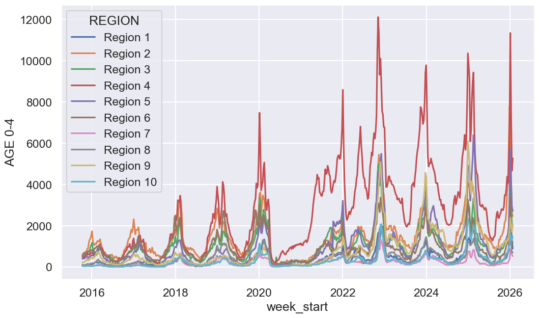
# Visualize overall prevalence of flu
f, ax = plt.subplots(1, 1, figsize=(12, 7))
sns.lineplot(ili, x='week_start', y='% WEIGHTED ILI', hue='REGION', ax=ax);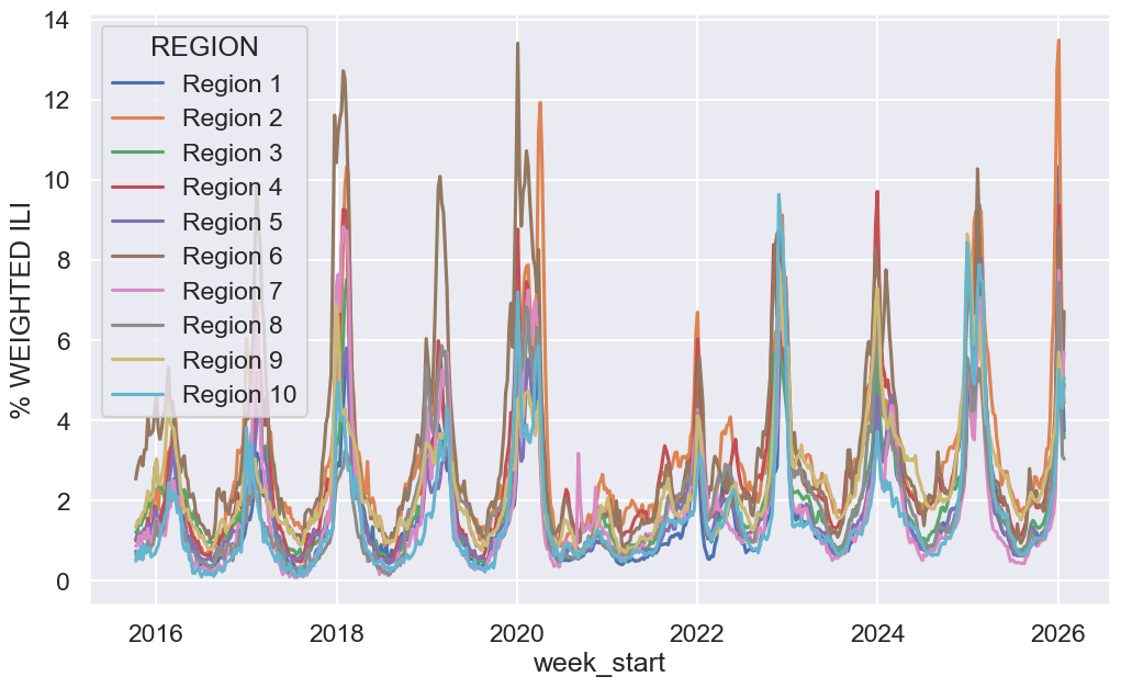
Take some time to examine it and consider any interesting observations or questions that arise from the data. We will explore data visualization in much more depth in upcoming lectures.
Load vaccination data
This DataFrame contains monthly flu vaccination counts for each flu season (starting in July and ending the following June).
Take a close look at the output, and make sure you understand what happens between 2023-06-01 and 2023-07-01!
vax = pd.read_csv('data/flu/monthly_child_flu_vaccination.csv')
vax['month_dt'] = pd.to_datetime(vax['month_dt'])
vax['rate'] = vax['Numerator'] / vax['Population']
vax.head(14)Joining Data (Merging different DataFrame)
First, let’s examine the two DataFrame we are merging.
display(ili.tail(2))
display(vax.tail(2))This is a natural point to pause and consider how weekly timestamps should be aggregated in order to match the monthly granularity of the vaccination data. In this example, we choose to associate each week with the month in which its start date falls. This isn’t the only way we could do this, and it also isn’t perfect: there may be weeks that are split across two months where the numbers won’t match up exactly.
ili["month"] = ili["week_start"].dt.to_period("M").dt.to_timestamp()Time to merge! Here we use the DataFrame method df1.merge(right=df2, ...) on DataFrame df1 (documentation). Contrast this with the function pd.merge(left=df1,right=df2, ...)(documentation). Feel free to use either.
ili_vax = ili.merge(
    vax,
    left_on=['month', 'REGION'],
    right_on=['month_dt', 'HHS Region']
)
ili_vax.head()We often merge datasets to get a much bigger picture of what’s really happening in the data—and one of the best ways to showcase that bigger picture is through a bigger visualization!
f, ax = plt.subplots(1, 1, figsize=(10, 7))
sns.scatterplot(ili_vax, x='ILITOTAL', y='rate', alpha=0.3, hue='HHS Region', ax=ax);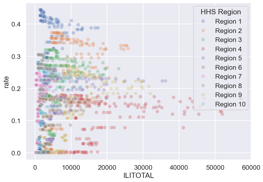
Hmm, this graph appears to show more information than the line plot we examined earlier, but something seems off. What are some limitations of this graph? We will explore what makes an effective visualization in more detail later.
Summary
We went over a lot of content this lecture; let’s summarize the most important points:
Dealing with Missing Values
There are a few options we can take to deal with missing data:
Drop missing records
Keep
NaNmissing valuesImpute using an interpolated column
EDA and Data Wrangling
There are several ways to approach EDA and Data Wrangling:
Examine the data and metadata: what is the date, size, organization, and structure of the data?
Examine each field/attribute/dimension individually.
Examine pairs of related dimensions (e.g. breaking down grades by major).
Along the way, we can:
Visualize or summarize the data.
Validate assumptions about data and its collection process. Pay particular attention to when the data was collected.
Identify and address anomalies.
Apply data transformations and corrections (we’ll cover this in the upcoming lecture).
Record everything you do! Developing in Jupyter Notebook promotes reproducibility of your own work!
[BONUS] EDA Demo 2: Mauna Loa CO2 Data – A Lesson in Data Faithfulness
We no longer cover the following demo in lecture, but we provide the following section in the course notes for interested students.
Mauna Loa Observatory has been monitoring CO2 concentrations since 1958.
co2_file = "data/co2_mm_mlo.txt"Let’s do some EDA!!
Reading this file into Pandas?
Let’s instead check out this .txt file. Some questions to keep in mind: Do we trust this file extension? What structure is it?
Lines 71-78 (inclusive) are shown below:
line number |                            file contents

71          |   #            decimal     average   interpolated    trend    #days
72          |   #             date                             (season corr)
73          |   1958   3    1958.208      315.71      315.71      314.62     -1
74          |   1958   4    1958.292      317.45      317.45      315.29     -1
75          |   1958   5    1958.375      317.50      317.50      314.71     -1
76          |   1958   6    1958.458      -99.99      317.10      314.85     -1
77          |   1958   7    1958.542      315.86      315.86      314.98     -1
78          |   1958   8    1958.625      314.93      314.93      315.94     -1
Notice how:
The values are separated by white space, possibly tabs.
The data line up down the rows. For example, the month appears in 7th to 8th position of each line.
The 71st and 72nd lines in the file contain column headings split over two lines.
We can use read_csv to read the data into a pandas DataFrame, and we provide several arguments to specify that the separators are white space, there is no header (we will set our own column names), and to skip the first 72 rows of the file.
co2 = pd.read_csv(
    co2_file, header = None, skiprows = 72,
    sep = r'\s+'       #delimiter for continuous whitespace (stay tuned for regex next lecture))
)
co2.head()Congratulations! You’ve wrangled the data!
...But our columns aren’t named. We need to do more EDA.
Exploring Variable Feature Types
The NOAA webpage might have some useful tidbits (in this case it doesn’t).
Using this information, we’ll rerun pd.read_csv, but this time with some custom column names.
co2 = pd.read_csv(
    co2_file, header = None, skiprows = 72,
    sep = r'\s+', #regex for continuous whitespace (next lecture)
    names = ['Yr', 'Mo', 'DecDate', 'Avg', 'Int', 'Trend', 'Days']
)
co2.head()Visualizing CO2
Scientific studies tend to have very clean data, right...? Let’s jump right in and make a time series plot of CO2 monthly averages.
sns.lineplot(x='DecDate', y='Avg', data=co2);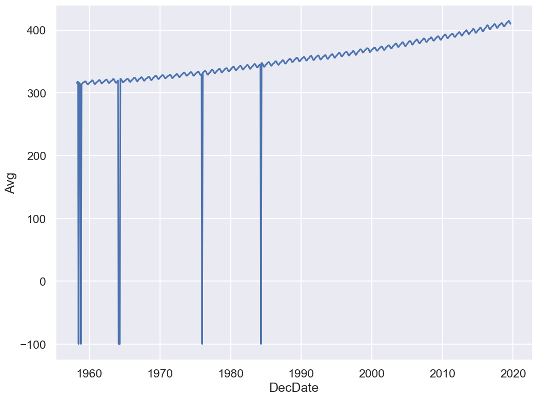
The code above uses the seaborn plotting library (abbreviated sns). We will cover this in the Visualization lecture, but now you don’t need to worry about how it works!
Yikes! Plotting the data uncovered a problem. The sharp vertical lines suggest that we have some missing values. What happened here?
co2.head()co2.tail()Some data have unusual values like -1 and -99.99.
Let’s check the description at the top of the file again.
-1 signifies a missing value for the number of days
Daysthe equipment was in operation that month.-99.99 denotes a missing monthly average
Avg
How can we fix this? First, let’s explore other aspects of our data. Understanding our data will help us decide what to do with the missing values.
Sanity Checks: Reasoning about the data
First, we consider the shape of the data. How many rows should we have?
If chronological order, we should have one record per month.
Data from March 1958 to August 2019.
We should have records.
co2.shape(738, 7)Nice!! The number of rows (i.e. records) match our expectations.
Let’s now check the quality of each feature.
Understanding Missing Value 1: Days
Days is a time field, so let’s analyze other time fields to see if there is an explanation for missing values of days of operation.
Let’s start with months, Mo.
Are we missing any records? The number of months should have 62 or 61 instances (March 1957-August 2019).
co2["Mo"].value_counts().sort_index()As expected Jan, Feb, Sep, Oct, Nov, and Dec have 61 occurrences and the rest 62.
Next let’s explore days Days itself, which is the number of days that the measurement equipment worked.
Click to see the code
sns.displot(co2['Days']);
plt.title("Distribution of days feature"); # suppresses unneeded plotting output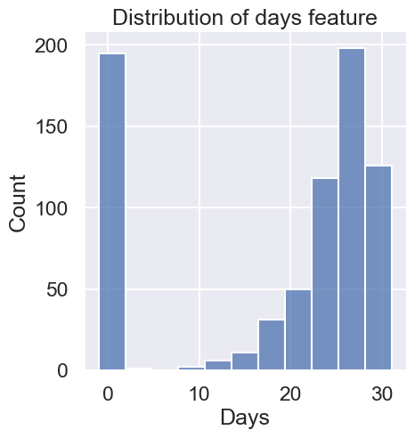
In terms of data quality, a handful of months have averages based on measurements taken on fewer than half the days. In addition, there are nearly 200 missing values--that’s about 27% of the data!
Finally, let’s check the last time feature, year Yr.
Let’s check to see if there is any connection between missing-ness and the year of the recording.
Click to see the code
sns.scatterplot(x="Yr", y="Days", data=co2);
plt.title("Day field by Year"); # the ; suppresses output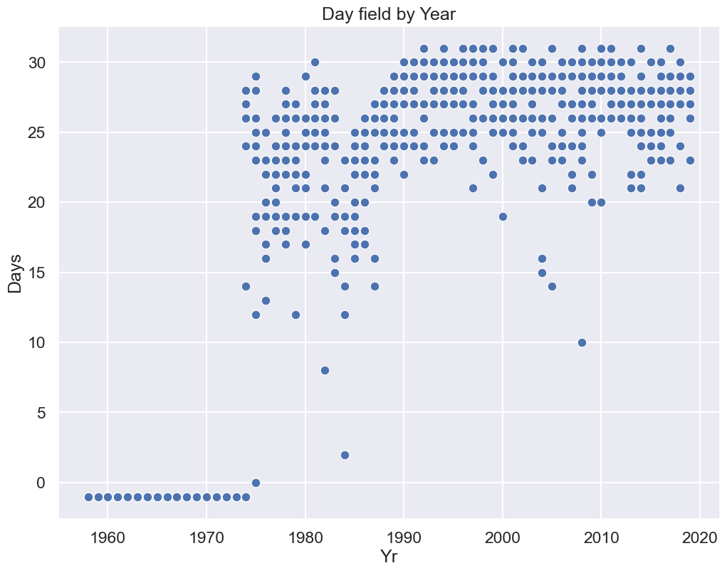
Observations:
All of the missing data are in the early years of operation.
It appears there may have been problems with equipment in the mid to late 80s.
Potential Next Steps:
Confirm these explanations through documentation about the historical readings.
Maybe drop the earliest recordings? However, we would want to delay such action until after we have examined the time trends and assess whether there are any potential problems.
Understanding Missing Value 2: Avg
Next, let’s return to the -99.99 values in Avg to analyze the overall quality of the CO2 measurements. We’ll plot a histogram of the average CO2 measurements
Click to see the code
# Histograms of average CO2 measurements
sns.displot(co2['Avg']);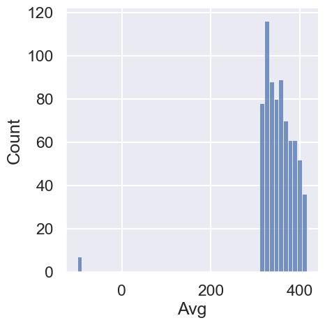
The non-missing values are in the 300-400 range (a regular range of CO2 levels).
We also see that there are only a few missing Avg values (<1% of values). Let’s examine all of them:
co2[co2["Avg"] < 0]There doesn’t seem to be a pattern to these values, other than that most records also were missing Days data.
Drop, NaN, or Impute Missing Avg Data?
How should we address the invalid Avg data?
Drop records
Set to NaN
Impute using some strategy
Remember we want to fix the following plot:
Click to see the code
sns.lineplot(x='DecDate', y='Avg', data=co2)
plt.title("CO2 Average By Month");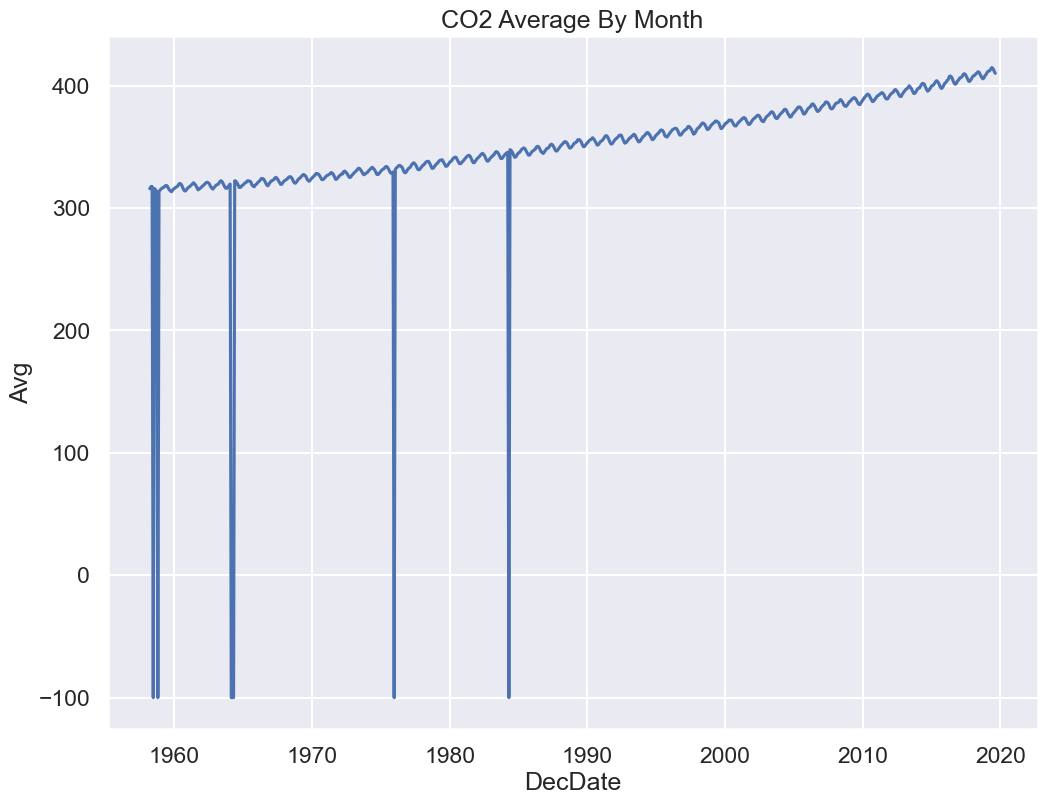
Since we are plotting Avg vs DecDate, we should just focus on dealing with missing values for Avg.
Let’s consider a few options:
Drop those records
Replace -99.99 with NaN
Substitute it with a likely value for the average CO2?
What do you think are the pros and cons of each possible action?
Let’s examine each of these three options.
# 1. Drop missing values
co2_drop = co2[co2['Avg'] > 0]
co2_drop.head()# 2. Replace NaN with -99.99
co2_NA = co2.replace(-99.99, np.nan)
co2_NA.head()We’ll also use a third version of the data.
First, we note that the dataset already comes with a substitute value for the -99.99.
From the file description:
The
interpolatedcolumn includes average values from the preceding column (average) and interpolated values where data are missing. Interpolated values are computed in two steps...
The Int feature has values that exactly match those in Avg, except when Avg is -99.99, and then a reasonable estimate is used instead.
So, the third version of our data will use the Int feature instead of Avg.
# 3. Use interpolated column which estimates missing Avg values
co2_impute = co2.copy()
co2_impute['Avg'] = co2['Int']
co2_impute.head()What’s a reasonable estimate?
To answer this question, let’s zoom in on a short time period, say the measurements in 1958 (where we know we have two missing values).
Click to see the code
# results of plotting data in 1958

def line_and_points(data, ax, title):
    # axssumes single year, hence Mo
    ax.plot('Mo', 'Avg', data=data)
    ax.scatter('Mo', 'Avg', data=data)
    ax.set_xlim(2, 13)
    ax.set_title(title)
    ax.set_xticks(np.arange(3, 13))

def data_year(data, year):
    return data[data["Yr"] == 1958]

# uses matplotlib subplots
# you may see more next week; focus on output for now
fig, axes = plt.subplots(ncols = 3, figsize=(12, 4), sharey=True)

year = 1958
line_and_points(data_year(co2_drop, year), axes[0], title="1. Drop Missing")
line_and_points(data_year(co2_NA, year), axes[1], title="2. Missing Set to NaN")
line_and_points(data_year(co2_impute, year), axes[2], title="3. Missing Interpolated")

fig.suptitle(f"Monthly Averages for {year}")
plt.tight_layout()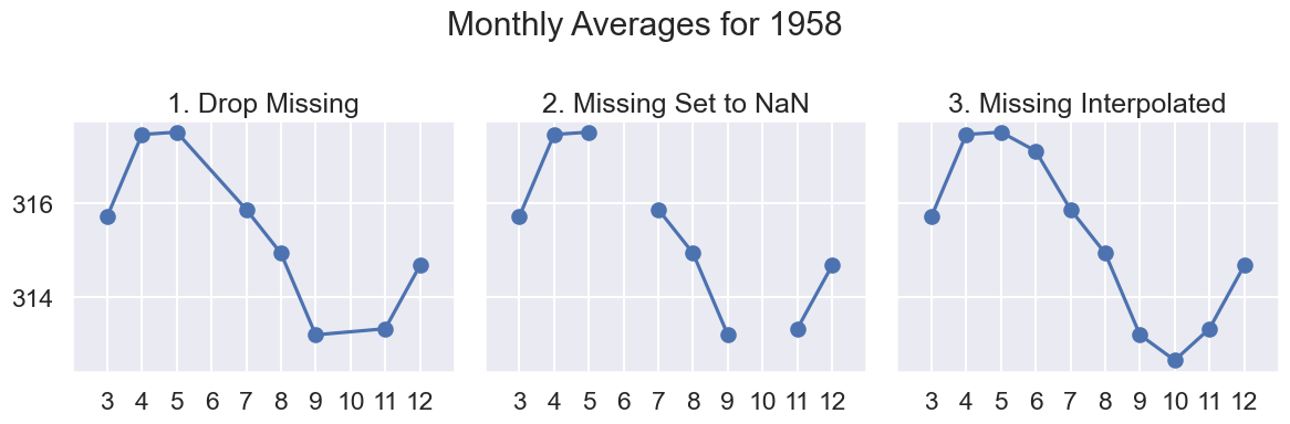
In the big picture since there are only 7 Avg values missing (<1% of 738 months), any of these approaches would work.
However there is some appeal to option C, Imputing:
Shows seasonal trends for CO2
We are plotting all months in our data as a line plot
Let’s replot our original figure with option 3:
Click to see the code
sns.lineplot(x='DecDate', y='Avg', data=co2_impute)
plt.title("CO2 Average By Month, Imputed");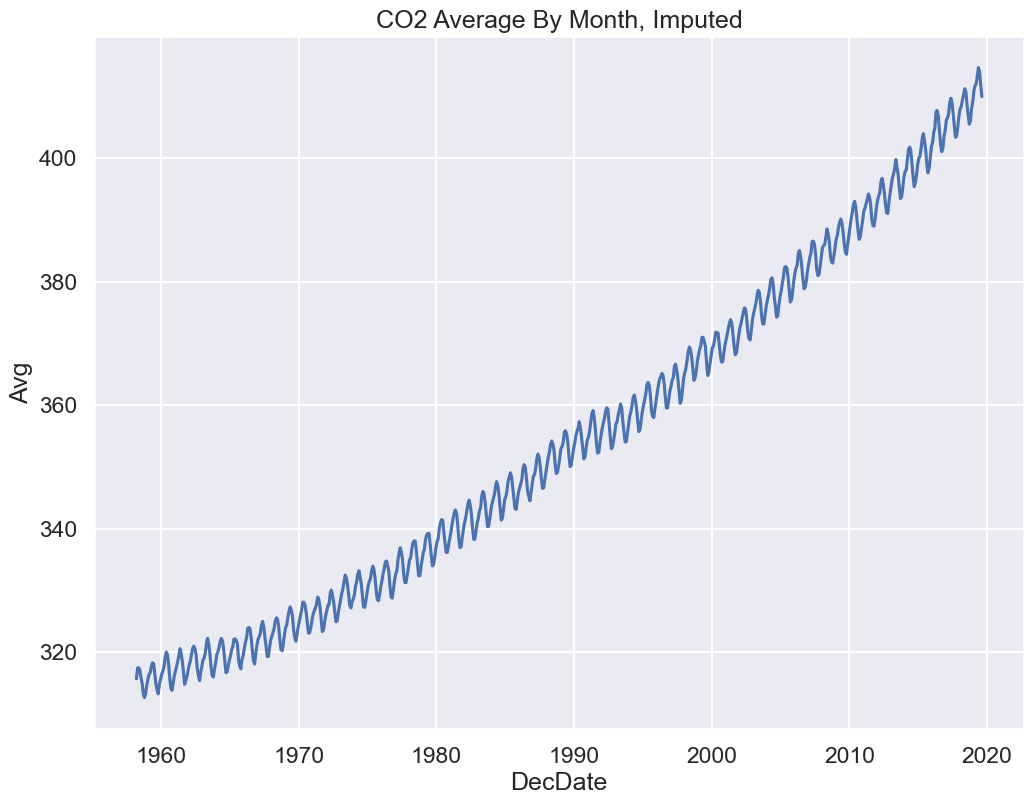
Looks pretty close to what we see on the NOAA website!
Presenting the Data: A Discussion on Data Granularity
From the description:
Monthly measurements are averages of average day measurements.
The NOAA GML website has datasets for daily/hourly measurements too.
The data you present depends on your research question.
How do CO2 levels vary by season?
You might want to keep average monthly data.
Are CO2 levels rising over the past 50+ years, consistent with global warming predictions?
You might be happier with a coarser granularity of average year data!
Click to see the code
co2_year = co2_impute.groupby('Yr').mean()
sns.lineplot(x='Yr', y='Avg', data=co2_year)
plt.title("CO2 Average By Year");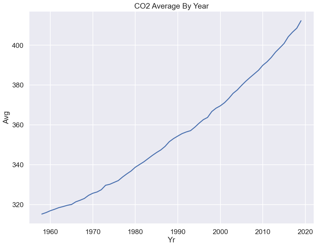
Indeed, we see a rise by nearly 100 ppm of CO2 since Mauna Loa began recording in 1958.