In this chapter, we will step back from the admissions case study and look at four properties every dataset has: its structure, granularity, temporality, and faithfulness. We will also combine tables with joins, and see why databases split data across many tables.
Key Data Properties
We ended last chapter by beginning to examine the following key data proprties:
Structure: the “shape” of a data file.
Granularity: how fine or coarse each datum is.
Temporality: how the data is situated in time.
Faithfulness: how well the data captures “reality”.
Structure has three parts here: the format a file arrives in, the type of each variable, and data that is spread across several tables. We started with an examination of data structure by discussing rectangular data and variable types. We will now turn to granularity. Afterwards, we will come back to structure in order to talk about combining tables with joins. We will then wrap up by discussing faithfulness and taking a look at how databases organize their tables.
Granularity
Granularity is what each record represents: a single purchase, a single person, a group of users. Fine-grained data has one row per small unit, such as one row per purchase. Coarse-grained data rolls many of those units up into each row, such as one row per customer with their total spending. Some datasets also include summaries, called rollups, as records next to the rows they summarize. If the data is coarse, ask how the records were aggregated: by summing, averaging, or something else. Coarse rows cannot be split back into finer ones, so a dataset’s granularity limits the questions it can answer.
Elections
What does each row of the elections dataset represent?
English: Read the elections data and preview it.
elections = pl.read_csv("data/elections.csv")
electionsThe shape header says the table has 187 rows. Each row names a year and a candidate, so a natural guess is that each row is one candidate in one election. We can test the guess by counting distinct values. .n_unique() on a Series, which EDA III used, counts the distinct values in one column.
elections["Year"].n_unique(), elections["Candidate"].n_unique(), elections.height(51, 135, 187)SQL:
SELECT COUNT(DISTINCT Year), COUNT(DISTINCT Candidate), COUNT(*)
FROM elections
COUNT(DISTINCT ...) counts distinct values instead of rows.
Neither column identifies a row by itself: there are 51 years and 135 candidates, against 187 rows. Andrew Jackson, for example, appears in 1824, 1828, and 1832. Called on a DataFrame, .n_unique() counts distinct rows, so after a select of two columns it counts the distinct combinations of their values.
English: Count the distinct combinations of year and candidate.
elections.select("Year", "Candidate").n_unique()187SQL:
SELECT COUNT(*)
FROM (SELECT DISTINCT Year, Candidate FROM elections)
SELECT DISTINCT keeps one copy of each distinct row, and the outer query counts them.
There are 187 distinct combinations of year and candidate, the same as the number of rows. Each row of elections represents a unique combination of candidate and year. That reading rests on two assumptions: there is at most one election in a year, and a candidate represents one party in each election.
Baby Names
The babynames dataset counts how many babies were given each name. Each of its rows represents a unique combination of name, state, sex, and year. Each count is itself a rollup: a row with a count of 5 stands for five individual births, which the dataset does not list one by one.
Admissions
The admissions table deserves the same check. EDA I noticed three schools named ABRAHAM LINCOLN HIGH SCHOOL, so a school’s name alone may not identify a row.
English: Count the distinct school names and the rows.
admissions["school"].n_unique(), admissions.height(1201, 1268)SQL:
SELECT COUNT(DISTINCT school), COUNT(*)
FROM admissions
There are 1201 distinct names for 1268 rows, so some names repeat.
English: Count the distinct combinations of school and city.
admissions.select("school", "city").n_unique()1268SQL:
SELECT COUNT(*)
FROM (SELECT DISTINCT school, city FROM admissions)
There are 1268 distinct combinations of school and city, one per row. A row of admissions is one school, identified by its name and its city together. Each row is also a rollup: its counts add up many individual decisions, by students to apply and attend and by the university to admit. That is why counts below 3 are blank (EDA I), since a count of one or two could reveal what happened to a single student.
Temporality
Temporality is how the data is situated in time. What type of variable is a datetime, such as 01/01/2025 3:30pm? People write datetimes as strings, and a first attempt might store them that way. Stored as strings, datetimes are hard to compare (“before” and “after”) and hard to compute with (“how long between”), and they take more space than numbers do. Here are three datetimes stored as strings.
Strings sort character by character, so 1950 lands between the two 2025 dates. 02/04/1950 comes after 01/01/2025 because 02 is greater than 01, and before 02/04/2025 because 19 is less than 20.
The fix is to parse each string into a datetime type that supports the kinds of calculations we wish to perform. Let us discuss the standard format for this.
Unix Time
A better way to store a datetime is as a number counted from an agreed origin. The computing standard is Unix time (also called POSIX time): the number of seconds since midnight on January 1, 1970, in Coordinated Universal Time (UTC). With every time stored as one number, “before”, “after”, and “how long between” become arithmetic.
polars has a datetime type, but working with this can be difficult. It is fine to use an LLM for help with these manipulations and calculations.
Structure Again: Data in Several Tables
Data often arrives spread across several files or tables. The admissions table we have used since EDA I is an example: the UC’s admissions counts were combined with enrollment and school information from the California Department of Education. The operation that combines them is a join. A join pairs the rows of two tables by a key, a column whose values say what each row is about, and the kind of join decides what happens to rows that have no partner.
Two Small Tables
To see each kind of join clearly, we use two tiny tables about cats. s holds each cat’s name and t holds each cat’s breed, and both are keyed by id.
s = pl.DataFrame({"id": [0, 1, 2, 4], "name": ["Apricot", "Boots", "Cally", "Eugene"]})
t = pl.DataFrame({"id": [1, 2, 4, 5], "breed": ["persian", "ragdoll", "bengal", "persian"]})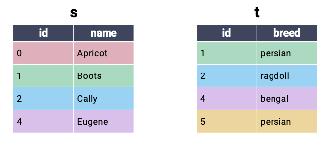
Ids 1, 2, and 4 appear in both tables. Id 0 (Apricot) appears only in s, and id 5 only in t.
Inner Join
An inner join combines each row of the first table with its matching row in the second table. A row that has no match is left out.
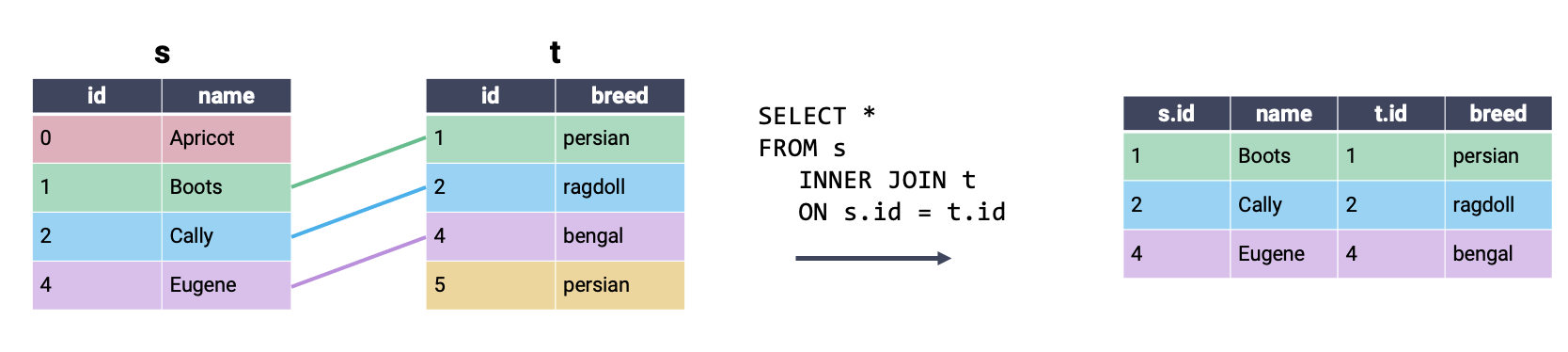
.join() takes the other table, the key column as on=, and the kind of join as how=.
English: For each cat, attach its breed, keeping only the cats that appear in both tables.
s.join(t, on="id", how="inner")SQL:
SELECT *
FROM s INNER JOIN t
    ON s.id = t.id
SQL specifies a join as part of the FROM clause: the kind of join (INNER JOIN), then the columns that decide which rows match (after ON). In Polars, how= gives the kind of join and on= the matching column. "inner" is the default, so s.join(t, on="id") gives the same result.
The result has 3 rows: Boots, Cally, and Eugene. Apricot and the id-5 persian have no partner, so they are dropped. The Polars result has a single id column, because on every row it keeps, the two tables’ ids are equal. The figure and the SQL’s SELECT * keep one id column from each table. For the full set of options, see the DataFrame.join documentation and the joins page of the Polars user guide.
Cross Join
A cross join pairs every row of the first table with every row of the second, and it is also called a Cartesian product. Nothing has to match, so a cross join needs no key, and on= is left out.
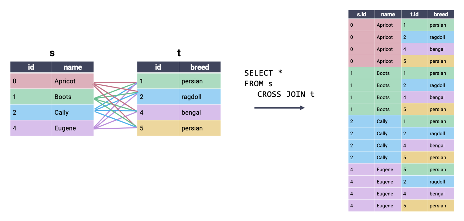
English: Pair every cat name with every breed.
s.join(t, how="cross")SQL:
SELECT *
FROM s CROSS JOIN t
The result has 4 × 4 = 16 rows. Both tables have a column named id, and a table cannot have two columns with the same name, so Polars keeps the left table’s column as id and renames the right table’s id_right. In general, Polars adds the suffix _right to any column of the right table whose name is already taken.
Inner Join as a Filtered Cross Join
The 16 rows include the 3 in which the two ids match. Keeping only those rows gives back the inner join.
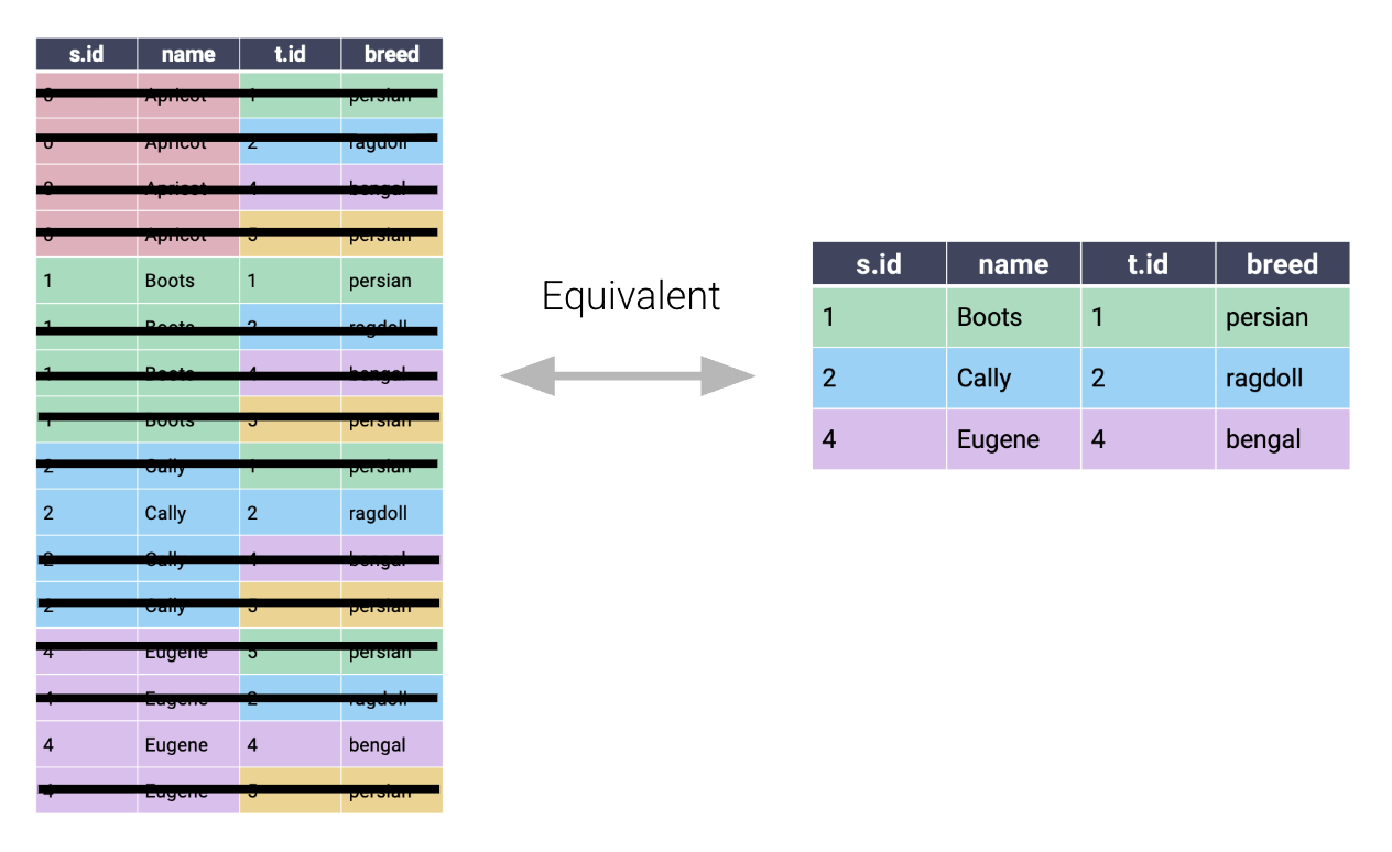
English: Keep the rows of the cross join whose two ids match.
matched = s.join(t, how="cross").filter(pl.col("id") == pl.col("id_right"))
matchedSQL:
SELECT *
FROM s CROSS JOIN t
WHERE s.id = t.id
This query returns the same rows as the inner join:
SELECT *
FROM s INNER JOIN t
    ON s.id = t.id
To check, we remove id_right with .drop(), which returns the table without the named columns, and compare the result with the inner join.
matched.drop("id_right").equals(s.join(t, on="id", how="inner"))TrueThis is a way to think about an inner join, not how a database computes one. Building every pair first would be far too slow on large tables.
Left Join
A left join (or left outer join) keeps every row of the left table, which is the first one named, and only the matching rows of the right table. Where a row of the left table has no match, the right table’s columns are filled with null.
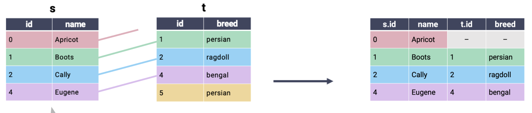
English: For each cat in s, attach its breed if t has one.
s.join(t, on="id", how="left")SQL:
SELECT *
FROM s LEFT JOIN t
    ON s.id = t.id
All 4 cats in s are kept, and Apricot’s breed is null, because t has no row with id 0. This null is a different kind of missing value from the ones in the section on faithfulness. Nothing was lost or suppressed: there was simply no partner to match.
Right Join
A right join is the mirror image. It keeps every row of the right table, the second one named, and fills in null where the left table has no match.
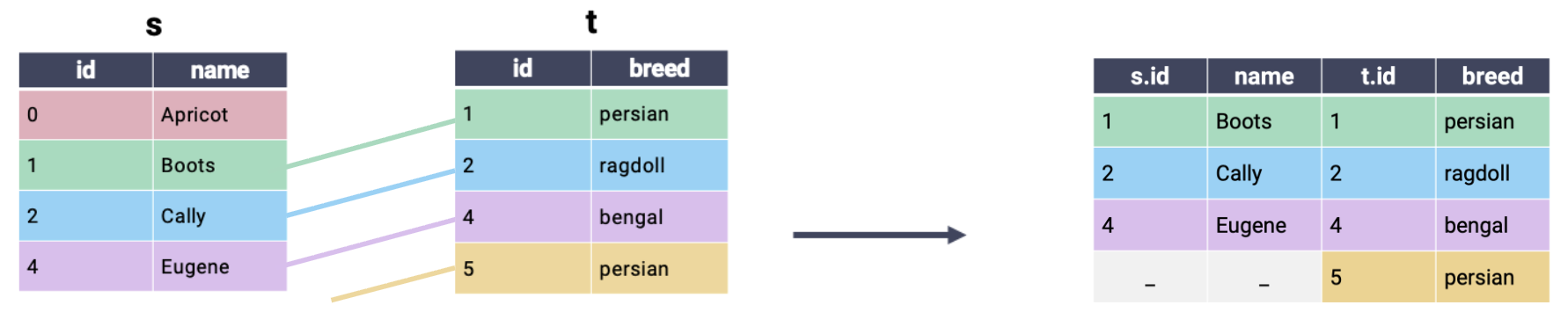
English: For each breed in t, attach the cat’s name if s has one.
s.join(t, on="id", how="right")SQL:
SELECT *
FROM s RIGHT JOIN t
    ON s.id = t.id
All 4 rows of t are kept, and the name for id 5 is null. Notice the column order in the Polars result, name, id, breed: the left table’s other columns come first, then the right table’s key and columns.
Full Outer Join
A full outer join keeps every row of both tables. It pairs the rows that match and fills in null wherever a row has no partner, much like doing a left join and a right join at once.
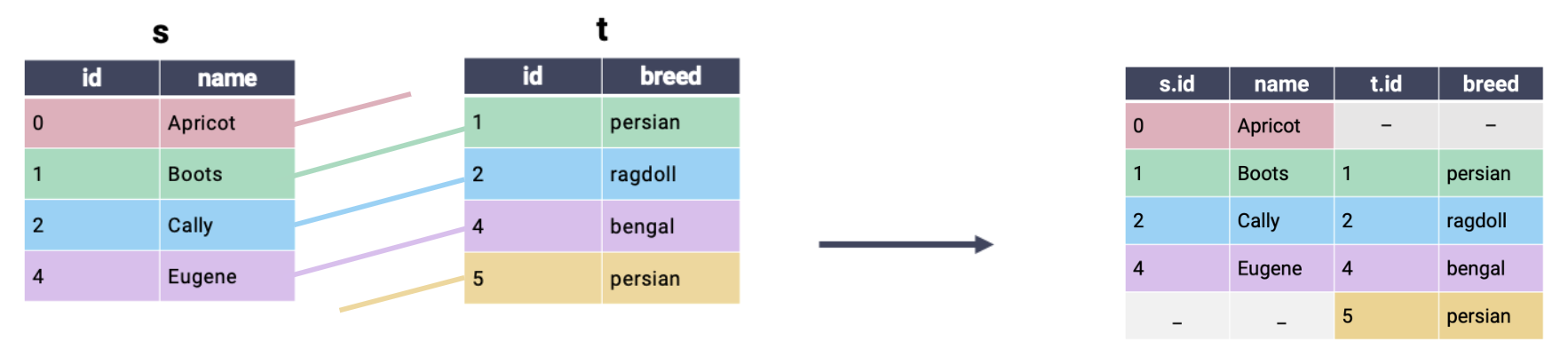
English: Keep every row from both tables, pairing names with breeds where the ids match.
s.join(t, on="id", how="full")SQL:
SELECT *
FROM s FULL JOIN t
    ON s.id = t.id
The result has 5 rows: the three matched cats, Apricot with no breed, and the id-5 persian with no name. This time Polars keeps both id and id_right, because each of them is null on one unmatched row: id is null on the persian’s row, and id_right on Apricot’s. Passing coalesce=True merges the two into a single id column, which takes whichever of the two values is not null.
s.join(t, on="id", how="full", coalesce=True)Now every row has an id. A join does not promise any particular row order, so refer to the rows of a join’s result by their key or name, not by their position. If you sort a full join on id without coalescing, pass nulls_last=True so that the unmatched right-table row does not sort to the top.
Equivalent Joins
Which of the queries A, B, and C return the same information as the first query below? Column order does not matter.
-- The query to match
SELECT * FROM s LEFT JOIN t ON s.id = t.id;

-- A
SELECT * FROM s LEFT JOIN t ON t.id = s.id;

-- B
SELECT * FROM t RIGHT JOIN s ON s.id = t.id;

-- C
SELECT * FROM s FULL JOIN t ON s.id = t.id WHERE s.id IS NOT NULL;
All three do.
A: the order of the two sides of an equality does not matter.
B: a right join is a left join with the tables named in the other order. Here
t’s columns come first.C: the full join adds the unmatched id-5 row, whose
s.idis null, and theWHEREclause removes it again.
B and C can be written in Polars too. B names t first and keeps every row of s:
t.join(s, on="id", how="right")It has the same 4 rows as the left join, with the columns in the order breed, id, name. C filters the full join down to the rows where s’s id, which Polars calls id, is not null:
s.join(t, on="id", how="full").filter(pl.col("id").is_not_null())It has the same 4 rows as the left join, plus the id_right column. A has no Polars counterpart, because on= names the key only once, so there is no equality to write in the other order.
Faithfulness
Faithfulness asks whether we can trust the data. How well does it reflect reality, and where might what the data says differ from what happened? Some questions to help answer that:
Are there any biases in the data collection process?
Who (or what) might not be represented in this data?
Would the data look different if someone else had collected it?
Why is the data grouped or sliced the way it is?
Were there limitations in the data-gathering process that matter?
Some faithfulness problems are visible in the data itself, and code can help find them.
Finding Problems in a Small Table
The table below is a small, made-up dataset of nine rows, small enough to read in full. Before reading on, look for anything that seems wrong.
Click to see the code
purchases = pl.DataFrame(
    {
        "ID": [0, 1, 2, 3, 4, 4, 5, 6, 7],
        "Category": ["Shoes", "Socks", "Socks", "Shirts", "Shoes", "Shoes", "Shirts", "Pnts", "Hats"],
        "State": ["CA", "NM", "XY", "NY", "FL", "FL", "CA", "TX", "CA"],
        "Location": ["CA", "NM", "XY", "NY", "FL", "FL", "CA", "TX", "CA"],
        "Device": [1, 1, 1, 1, 1, 1, 1, 1, 1],
        "Purchased": [1, 0, 0, None, 0, 0, 0, 1, -1],
    }
)
purchases
Here are some issues with this data:
There are two rows that are exact duplicates
There is row with an “XY” state abbreviation
The “Device” column is always 1
What does it mean for “Purchased” value to be “None” or -1?
One of the rows has a “Pnts” value for the “Category” column, which appears to be a typo
Note that we are only looking at eight rows of this data, so any conclusions we draw may not hold for the rest of the data. For example, it is possible that the “Device” column takes on values other than 1 in other rows.
In general:
Fully Duplicated Records or Fields
Ignore/drop, if no reason for duplication.
Labeling or Spelling Errors
Apply corrections. Only ignore if you have to.
Missing data
Need to think carefully about why the data is missing.
How Missing Values Are Encoded
Missing data does not always look missing. Some common encodings:
| Encoding | Examples |
|---|---|
| A blank or a space | "", " " |
| A sentinel number | 0, -1999, 12345 |
| Not a Number | NaN |
| A missing-value marker | null, NA |
| A default date | 1970, 2000 |
A default date of January 1, 1970 is often a Unix time of 0 standing in for “unknown”. A single column can even hold a real 0 in some rows and a placeholder 0 in others. Before deciding how to handle missing values, work out how they were encoded and why they are missing.
How To Handle Missing Values
Here are some approaches to handling missing values:
Keep as null
A good default
If qualitative/categorical, consider creating a “Missing” category
Drop records with missing values
Typically a bad default!
If a temparature probe went offline for a minute, then it is likely missing at random, and okay to drop
If a police officer never records of outcomes of vehicle stops, then it is likely not missing at random, and holds valuable information
Imputation/interpolation: Infer missing values
Mean/median imputation
Mode imputation
Hot deck imputation: Use a random non-null value
We did this when selecting a random number between 0 and 2 (inclusive), but this is largely out of scope for this course
There are others, but they are out of scope for this course
Structure: File Formats
A file format is an agreement about where one record ends and the next begins, and where one field ends and the next begins. When a file follows the usual agreement, reading it takes one line of code. When it breaks the agreement, we have to tell the reader what the file does instead. We will read three common formats: CSV, TSV, and JSON.
CSV And TSV Files
In a CSV (comma-separated values) file, records (entries/rows) are separated by newlines (\n) and fields (features/columns) are separated by commas (,). The first row contains the headers (feature/column names), also separated by commas.
A TSV file is organized in basically the same way as a CSV file, except that the headers and fields are separated by tabs (\t).
Both are largely rectangular, but the rows are not required to have the same number of fields. There may not be more fields than headers, and parsers usually fill in blank fields in a given row with null values.
You can open CSV and TSV files in polars using pl.read_csv(), such as for this file of tuberculosis records by state:
tb_tsv = pl.read_csv("data/cdc_tuberculosis.tsv", separator="\t")tb_tsv.head()If you look at the separator= parameter, you will see that we entered the delimiter for TSV files. For CSV files, you would use separator=',' instead. You can learn more about different parameters at the documention for pl.read_csv().
JSON Files
JSON files resemble Python dictionaries. Each record has its own item, with key: value pairs for each field. The key will be a field name, with the corresponding value often being that record’s value for the given field. This structure means that the field names are repeated for every record, unlike CSV and TSV files (where the fields are only named in the first row containing the headers).
The reason we say “often” is that JSON files can contain nested dicitonaries. In these cases, a field name key can be assigned another dictionary of sub-fields as its value. An example could be a dataset of rooms in a school, with a field named “Measurements” that contains two sub-fields named “Floor Area” and “Ceiling Height”.
JSON files are not necessarily rectangular, given the nested structure. Some fields or sub-fields may not be present for all records.
We can read in JSON files using pl.read_json(). You can find further information in the documentation.
Databases: Why SQL?
Every table in this chapter so far came from a file. In practice, much of the data a data scientist works with lives in a database instead. A database is an organized collection of data. A database management system (DBMS) is a software system that stores, manages, and gives access to one or more databases. Common large-scale DBMSs in data science include Google BigQuery, Amazon Redshift, Snowflake, Databricks, and Microsoft SQL Server.
Why not keep everything in CSV files? A DBMS has advantages in two areas.
Data storage
Reliable storage that survives system crashes and disk failures.
Computation on data that does not fit in memory.
Special data structures that improve performance (covered in CS 186).
Data management
Control over how the data is logically organized and who has access to it.
Guarantees on the data, such as a person’s age never being negative, which prevent data anomalies.
Safe concurrent operations, so that many users can read and write the data at the same time, as they do with ATM transactions.
EDA I described a typical EDA workflow: a database with many dynamic tables, updated frequently (after every customer purchase, for example); a few snapshotted tables, pulled from it with SQL as they stood at one moment in time; manipulation of those snapshots with Polars (or R, pandas, or Excel); and visualization with seaborn. This section is about the first step, the database.
Data scientists use SQL in a few main ways:
Write a SQL query to get the initial dataset for an analysis, save it as a CSV (or JSON, or another format), and explore and analyze it with Polars.
Interact with the DBMS directly: write SQL queries to explore and analyze the data, save the final results to a CSV, and make figures and summaries with Polars or other tools.
Use an ORM (object-relational mapping), which translates Python code into SQL automatically. ORMs are most common in large software systems and less common in data science.
Write SQL queries that run automatically on a schedule, a semi-automated version of the second approach.
Here is the first approach on a small scale. We are hiding the code, as you are not required to memorize this. You can also find additional info in the collapsed note below.
OPTIONAL: How To Use SQL In Python
DuckDB is a DBMS that runs inside Python and keeps a whole database in a single file. duckdb.connect opens that file and returns a connection to it, and pl.read_database sends a SQL query over the connection and returns the result as a DataFrame. Opening the file with read_only=True means that nothing we do can change it. Writing queries of your own is the subject of the SQL chapters, so here we only fetch two whole tables.
Source
import duckdb

con = duckdb.connect("data/example_duck.db", read_only=True)
dragon = pl.read_database("SELECT * FROM dragon", con)
setting = pl.read_database("SELECT * FROM setting", con)dragonSQL has its own names for the parts of a table.
A table is also called a relation, and
dragonis the relation’s name.A row is also called a record or a tuple.
A column is also called an attribute or a field.
The dragon relation has 6 records, one per dragon, and 4 attributes: name, yr, cute, and setting_id.
Table Schema
Every column of a SQL table has three properties: a name, a type, and zero or more constraints, which are rules that every value in the column must obey. The schema of a DataFrame has only the first two.
English: List each column of dragon with its type.
dragon.schemaSchema([('name', String),
('yr', Int64),
('cute', Int64),
('setting_id', Int64)])SQL:
DESCRIBE dragonThe Polars schema records names and types (String and Int32), and nothing else. In a database, whoever creates a table must declare its schema, which describes the logical structure of the table, and the constraints are part of that declaration. These are the two statements that created the tables in example_duck.db, with setting first because dragon refers to it:
CREATE TABLE setting (
    id         INTEGER PRIMARY KEY,
    media      VARCHAR NOT NULL,
    place      VARCHAR,
    "type"     VARCHAR,
    start_year INTEGER,
    CHECK (start_year >= 1900)
);

CREATE TABLE dragon (
    "name"     VARCHAR PRIMARY KEY,
    yr         INTEGER,
    cute       INTEGER,
    setting_id INTEGER,
    CHECK (yr >= 1900),
    FOREIGN KEY (setting_id) REFERENCES setting(id)
);
Each line gives a column’s name and type, then any constraints on it. VARCHAR is text, and INTEGER is a 32-bit integer, which is why Polars shows i32. (name and type are in double quotes because they are also SQL keywords.) The constraints are:
PRIMARY KEY: the column identifies each row. Every row must have a value, and no two rows may share one.NOT NULL: every row must have a value, so a setting cannot be missing itsmedia.CHECK (yr >= 1900): a dragon’s year cannot be before 1900.settinghas the same rule forstart_year.FOREIGN KEY (setting_id) REFERENCES setting(id): each dragon’ssetting_idmust be either null or anidthat exists insetting.
The database refuses any change that would break a constraint. That is the “guarantees on the data” advantage of a DBMS, written out in code.
Why Multiple Tables?
Suppose we want to know where each dragon comes from. That information lives in the setting table.
settingsetting has 5 rows, one per setting, identified by id. Each row records the title of the work the setting comes from (media), the place, the type of work, and the year the work first appeared (start_year). The setting with id 2, IRL (“in real life”), has no place and no start year.
To attach each dragon’s setting, we join the two tables, matching dragon’s setting_id with setting’s id. The key has a different name in each table, so instead of on= we name the left table’s key with left_on= and the right table’s with right_on=.
English: For each dragon, attach its setting.
dragon.join(setting, left_on="setting_id", right_on="id")SQL:
SELECT *
FROM dragon INNER JOIN setting
    ON dragon.setting_id = setting.id
The result has 6 rows and 8 columns. Polars keeps setting_id and drops id, since the two are equal on every row, while the SQL result keeps both and has 9 columns.
This wide table is what we would get by storing everything about dragons in one table, and it shows two problems with doing that.
Redundant information. drogon and rhaegal both come from Game of Thrones, so the table stores
Game of Thrones,Essos,tv show, and2011twice. Every dragon from the same setting repeats all of that setting’s information.Column bloat. Half of the columns,
media,place,type, andstart_year, describe settings rather than dragons. As we add more about each setting, the table stops being about dragons at all.
The solution is to split the information into several tables, store each fact once, and join the tables whenever an analysis needs them together.
Primary and Foreign Keys
A primary key is a column (or set of columns) that identifies each row of a table. The primary key of dragon is name, so no two dragons may share a name.
English: Check that every dragon has a different name.
dragon["name"].n_unique(), dragon.height(6, 6)SQL:
SELECT COUNT(DISTINCT name), COUNT(*)
FROM dragon
There are 6 distinct names in 6 rows. A check like this shows only that the rows we have are unique; the PRIMARY KEY constraint is what guarantees that no future row will repeat a name. A key can also span several columns. In the section on granularity, school and city together identified each row of admissions.
The primary key of setting is id. A foreign key is a column that holds another table’s primary keys. setting_id in dragon is a foreign key into setting: it records which setting each dragon comes from, without repeating any of that setting’s information. Foreign keys are usually what we join on. The join above kept all 6 dragons. No dragon has a null setting_id, and the foreign-key constraint guarantees that every non-null setting_id appears as an id in setting. A dragon with a null setting_id would pass the constraint, and an inner join would drop it.
Star Schema
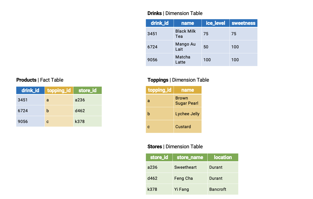
To minimize redundant storage, databases often store data across fact and dimension tables. This arrangement is called a star schema, and the figure shows one for a group of boba shops.
The fact table is the central table, and it holds the information that links its entries to the dimension tables. It has few columns and many records. Here,
Productsholds only keys:drink_id,topping_id, andstore_id.Each dimension table holds more detailed information about one kind of fact. Dimension tables have more columns and fewer records.
Drinkshas each drink’s name, ice level, and sweetness;Toppingshas each topping’s name; andStoreshas each store’s name and location.
The fact table’s granularity is every possible drink and topping combination across all stores, which makes for many rows. With the 3 drinks, 3 toppings, and 3 stores in the figure, there are 3 × 3 × 3 = 27 combinations: the cross join of the three dimension tables’ keys. To see a drink’s name next to the location of a store that sells it, we join Products with Drinks on drink_id and with Stores on store_id. Each description is stored once, and joins bring together whatever an analysis needs.
Parting Note
Structure, granularity, temporality, and faithfulness are questions to carry into any dataset. What shape is the data in, and what does one row represent? When was it recorded, and in which time zone? Does it reflect reality, and how are its missing values encoded?
It is also important to become familiar with SQL, as well as database management systems more broadly. These are your method of accessing information from large databases, particularly ones that are regularly updated (requiring you to take a snapshot of the data at a particular time).
Next, we will dive into regular expressions, also known as Regex.