Use the pd.pivot_table method to contruct a pivot table
Perform simple merges between DataFrames using pd.merge()
4.1GroupBy(), Continued
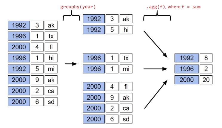
As we learned last lecture, a groupby operation involves some combination of splitting a DataFrame into grouped subframes, applying a function, and combining the results.
For some arbitrary DataFrame df below, the code df.groupby("year").agg(sum) does the following:
Splits the DataFrame into sub-DataFrames with rows belonging to the same year.
Applies the sum function to each column of each sub-DataFrame.
Combines the results of sum into a single DataFrame, indexed by year.
4.1.1 Aggregation with lambda Functions
We’ll work with the elections DataFrame again.
Code
import pandas as pdimport numpy as npelections = pd.read_csv("data/elections.csv")elections.head(5)
Year
Candidate
Party
Popular vote
Result
%
0
1824
Andrew Jackson
Democratic-Republican
151271
loss
57.210122
1
1824
John Quincy Adams
Democratic-Republican
113142
win
42.789878
2
1828
Andrew Jackson
Democratic
642806
win
56.203927
3
1828
John Quincy Adams
National Republican
500897
loss
43.796073
4
1832
Andrew Jackson
Democratic
702735
win
54.574789
What if we wish to aggregate our DataFrame using a non-standard function – for example, a function of our own design? We can do so by combining .agg with lambda expressions.
Let’s first consider a puzzle to jog our memory. We will attempt to find the Candidate from each Party with the highest % of votes.
A naive approach may be to group by the Party column and aggregate by the maximum.
elections.groupby("Party").agg(max).head(10)
Year
Candidate
Popular vote
Result
%
Party
American
1976
Thomas J. Anderson
873053
loss
21.554001
American Independent
1976
Lester Maddox
9901118
loss
13.571218
Anti-Masonic
1832
William Wirt
100715
loss
7.821583
Anti-Monopoly
1884
Benjamin Butler
134294
loss
1.335838
Citizens
1980
Barry Commoner
233052
loss
0.270182
Communist
1932
William Z. Foster
103307
loss
0.261069
Constitution
2016
Michael Peroutka
203091
loss
0.152398
Constitutional Union
1860
John Bell
590901
loss
12.639283
Democratic
2020
Woodrow Wilson
81268924
win
61.344703
Democratic-Republican
1824
John Quincy Adams
151271
win
57.210122
This approach is clearly wrong – the DataFrame claims that Woodrow Wilson won the presidency in 2020.
Why is this happening? Here, the max aggregation function is taken over every column independently. Among Democrats, max is computing:
The most recent Year a Democratic candidate ran for president (2020)
The Candidate with the alphabetically “largest” name (“Woodrow Wilson”)
The Result with the alphabetically “largest” outcome (“win”)
Instead, let’s try a different approach. We will:
Sort the DataFrame so that rows are in descending order of %
Group by Party and select the first row of each sub-DataFrame
While it may seem unintuitive, sorting elections by descending order of % is extremely helpful. If we then group by Party, the first row of each groupby object will contain information about the Candidate with the highest voter %.
elections_sorted_by_percent.groupby("Party").agg(lambda x : x.iloc[0]).head(10)# Equivalent to the below code# elections_sorted_by_percent.groupby("Party").agg('first').head(10)
Year
Candidate
Popular vote
Result
%
Party
American
1856
Millard Fillmore
873053
loss
21.554001
American Independent
1968
George Wallace
9901118
loss
13.571218
Anti-Masonic
1832
William Wirt
100715
loss
7.821583
Anti-Monopoly
1884
Benjamin Butler
134294
loss
1.335838
Citizens
1980
Barry Commoner
233052
loss
0.270182
Communist
1932
William Z. Foster
103307
loss
0.261069
Constitution
2008
Chuck Baldwin
199750
loss
0.152398
Constitutional Union
1860
John Bell
590901
loss
12.639283
Democratic
1964
Lyndon Johnson
43127041
win
61.344703
Democratic-Republican
1824
Andrew Jackson
151271
loss
57.210122
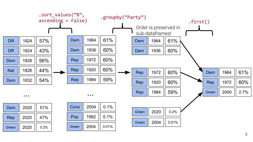
Here’s an illustration of the process:
Notice how our code correctly determines that Lyndon Johnson from the Democratic Party has the highest voter %.
More generally, lambda functions are used to design custom aggregation functions that aren’t pre-defined by Python. The input parameter x to the lambda function is a GroupBy object. Therefore, it should make sense why lambda x : x.iloc[0] selects the first row in each groupby object.
In fact, there’s a few different ways to approach this problem. Each approach has different tradeoffs in terms of readability, performance, memory consumption, complexity, etc. We’ve given a few examples below.
Note: Understanding these alternative solutions is not required. They are given to demonstrate the vast number of problem-solving approaches in pandas.
# Using the idxmax functionbest_per_party = elections.loc[elections.groupby('Party')['%'].idxmax()]best_per_party.head(5)
Year
Candidate
Party
Popular vote
Result
%
22
1856
Millard Fillmore
American
873053
loss
21.554001
115
1968
George Wallace
American Independent
9901118
loss
13.571218
6
1832
William Wirt
Anti-Masonic
100715
loss
7.821583
38
1884
Benjamin Butler
Anti-Monopoly
134294
loss
1.335838
127
1980
Barry Commoner
Citizens
233052
loss
0.270182
# Using the .drop_duplicates functionbest_per_party2 = elections.sort_values('%').drop_duplicates(['Party'], keep='last')best_per_party2.head(5)
Year
Candidate
Party
Popular vote
Result
%
148
1996
John Hagelin
Natural Law
113670
loss
0.118219
164
2008
Chuck Baldwin
Constitution
199750
loss
0.152398
110
1956
T. Coleman Andrews
States' Rights
107929
loss
0.174883
147
1996
Howard Phillips
Taxpayers
184656
loss
0.192045
136
1988
Lenora Fulani
New Alliance
217221
loss
0.237804
4.1.2 Other GroupBy Features
There are many aggregation methods we can use with .agg. Some useful options are:
.mean: creates a new DataFrame with the mean value of each group
.sum: creates a new DataFrame with the sum of each group
.max and .min: creates a new DataFrame with the maximum/minimum value of each group
.first and .last: creates a new DataFrame with the first/last row in each group
.size: creates a new Series with the number of entries in each group
.count: creates a new DataFrame with the number of entries, excluding missing values.
Note the slight difference between .size() and .count(): while .size() returns a Series and counts the number of entries including the missing values, .count() returns a DataFrame and counts the number of entries in each column excluding missing values. Here’s an example:
You might recall that the value_counts() function in the previous note does something similar. It turns out value_counts() and groupby.size() are the same, except value_counts() sorts the resulting Series in descending order automatically.
df["letter"].value_counts()
letter
C    3
A    2
B    1
Name: count, dtype: int64
These (and other) aggregation functions are so common that pandas allows for writing shorthand. Instead of explicitly stating the use of .agg, we can call the function directly on the GroupBy object.
For example, the following are equivalent:
elections.groupby("Candidate").agg(mean)
elections.groupby("Candidate").mean()
There are many other methods that pandas supports. You can check them out on the pandas documentation.
4.1.3 Filtering by Group
Another common use for GroupBy objects is to filter data by group.
groupby.filter takes an argument \(\text{f}\), where \(\text{f}\) is a function that:
Takes a DataFrame object as input
Returns a single True or False for the each sub-DataFrame
Sub-DataFrames that correspond to True are returned in the final result, whereas those with a False value are not. Importantly, groupby.filter is different from groupby.agg in that an entire sub-DataFrame is returned in the final DataFrame, not just a single row. As a result, groupby.filter preserves the original indices.
To illustrate how this happens, consider the following .filter function applied on some arbitrary data. Say we want to identify “tight” election years – that is, we want to find all rows that correspond to elections years where all candidates in that year won a similar portion of the total vote. Specifically, let’s find all rows corresponding to a year where no candidate won more than 45% of the total vote.
In other words, we want to:
Find the years where the maximum % in that year is less than 45%
Return all DataFrame rows that correspond to these years
For each year, we need to find the maximum % among all rows for that year. If this maximum % is lower than 45%, we will tell pandas to keep all rows corresponding to that year.
What’s going on here? In this example, we’ve defined our filtering function, \(\text{f}\), to be lambda sf: sf["%"].max() < 45. This filtering function will find the maximum "%" value among all entries in the grouped sub-DataFrame, which we call sf. If the maximum value is less than 45, then the filter function will return True and all rows in that grouped sub-DataFrame will appear in the final output DataFrame.
Examine the DataFrame above. Notice how, in this preview of the first 9 rows, all entries from the years 1860 and 1912 appear. This means that in 1860 and 1912, no candidate in that year won more than 45% of the total vote.
You may ask: how is the groupby.filter procedure different to the boolean filtering we’ve seen previously? Boolean filtering considers individual rows when applying a boolean condition. For example, the code elections[elections["%"] < 45] will check the "%" value of every single row in elections; if it is less than 45, then that row will be kept in the output. groupby.filter, in contrast, applies a boolean condition across all rows in a group. If not all rows in that group satisfy the condition specified by the filter, the entire group will be discarded in the output.
4.2 Aggregating Data with Pivot Tables
We know now that .groupby gives us the ability to group and aggregate data across our DataFrame. The examples above formed groups using just one column in the DataFrame. It’s possible to group by multiple columns at once by passing in a list of column names to .groupby.
Let’s consider the babynames dataset. In this problem, we will find the total number of baby names associated with each sex for each year. To do this, we’ll group by both the "Year" and "Sex" columns.
Code
import urllib.requestimport os.path# Download data from the web directlydata_url ="https://www.ssa.gov/oact/babynames/names.zip"local_filename ="data/babynames.zip"ifnot os.path.exists(local_filename): # if the data exists don't download againwith urllib.request.urlopen(data_url) as resp, open(local_filename, 'wb') as f: f.write(resp.read())# Load data without unzipping the fileimport zipfilebabynames = [] with zipfile.ZipFile(local_filename, "r") as zf: data_files = [f for f in zf.filelist if f.filename[-3:] =="txt"]def extract_year_from_filename(fn):returnint(fn[3:7])for f in data_files: year = extract_year_from_filename(f.filename)with zf.open(f) as fp: df = pd.read_csv(fp, names=["Name", "Sex", "Count"]) df["Year"] = year babynames.append(df)babynames = pd.concat(babynames)
babynames.head()
Name
Sex
Count
Year
0
Mary
F
7065
1880
1
Anna
F
2604
1880
2
Emma
F
2003
1880
3
Elizabeth
F
1939
1880
4
Minnie
F
1746
1880
# Find the total number of baby names associated with each sex for each year in the datababynames.groupby(["Year", "Sex"])[["Count"]].agg(sum).head(6)
Count
Year
Sex
1880
F
90994
M
110490
1881
F
91953
M
100737
1882
F
107847
M
113686
Notice that both "Year" and "Sex" serve as the index of the DataFrame (they are both rendered in bold). We’ve created a multi-index DataFrame where two different index values, the year and sex, are used to uniquely identify each row.
This isn’t the most intuitive way of representing this data – and, because multi-indexed DataFrames have multiple dimensions in their index, they can often be difficult to use.
Another strategy to aggregate across two columns is to create a pivot table. You saw these back in Data 8. One set of values is used to create the index of the pivot table; another set is used to define the column names. The values contained in each cell of the table correspond to the aggregated data for each index-column pair.
The best way to understand pivot tables is to see one in action. Let’s return to our original goal of summing the total number of names associated with each combination of year and sex. We’ll call the pandas.pivot_table method to create a new table.
# The `pivot_table` method is used to generate a Pandas pivot tableimport numpy as npbabynames.pivot_table( index ="Year", columns ="Sex", values ="Count", aggfunc = np.sum).head(5)
Sex
F
M
Year
1880
90994
110490
1881
91953
100737
1882
107847
113686
1883
112319
104625
1884
129019
114442
Looks a lot better! Now, our DataFrame is structured with clear index-column combinations. Each entry in the pivot table represents the summed count of names for a given combination of "Year" and "Sex".
Let’s take a closer look at the code implemented above.
index = "Year" specifies the column name in the original DataFrame that should be used as the index of the pivot table
columns = "Sex" specifies the column name in the original DataFrame that should be used to generate the columns of the pivot table
values = "Count" indicates what values from the original DataFrame should be used to populate the entry for each index-column combination
aggfunc = np.sum tells pandas what function to use when aggregating the data specified by values. Here, we are summing the name counts for each pair of "Year" and "Sex"
We can even include multiple values in the index or columns of our pivot tables.
babynames_pivot = babynames.pivot_table( index="Year", # the rows (turned into index) columns="Sex", # the column values values=["Count", "Name"], aggfunc=max, # group operation)babynames_pivot.head(6)
Count
Name
Sex
F
M
F
M
Year
1880
7065
9655
Zula
Zeke
1881
6919
8769
Zula
Zeb
1882
8148
9557
Zula
Zed
1883
8012
8894
Zula
Zeno
1884
9217
9388
Zula
Zollie
1885
9128
8756
Zula
Zollie
4.3 Joining Tables
When working on data science projects, we’re unlikely to have absolutely all the data we want contained in a single DataFrame – a real-world data scientist needs to grapple with data coming from multiple sources. If we have access to multiple datasets with related information, we can join two or more tables into a single DataFrame.
To put this into practice, we’ll revisit the elections dataset.
elections.head(5)
Year
Candidate
Party
Popular vote
Result
%
0
1824
Andrew Jackson
Democratic-Republican
151271
loss
57.210122
1
1824
John Quincy Adams
Democratic-Republican
113142
win
42.789878
2
1828
Andrew Jackson
Democratic
642806
win
56.203927
3
1828
John Quincy Adams
National Republican
500897
loss
43.796073
4
1832
Andrew Jackson
Democratic
702735
win
54.574789
Say we want to understand the popularity of the names of each presidential candidate in 2020. To do this, we’ll need the combined data of babynamesandelections.
We’ll start by creating a new column containing the first name of each presidential candidate. This will help us join each name in elections to the corresponding name data in babynames.
# This `str` operation splits each candidate's full name at each # blank space, then takes just the candidiate's first nameelections["First Name"] = elections["Candidate"].str.split().str[0]elections.head(5)
Year
Candidate
Party
Popular vote
Result
%
First Name
0
1824
Andrew Jackson
Democratic-Republican
151271
loss
57.210122
Andrew
1
1824
John Quincy Adams
Democratic-Republican
113142
win
42.789878
John
2
1828
Andrew Jackson
Democratic
642806
win
56.203927
Andrew
3
1828
John Quincy Adams
National Republican
500897
loss
43.796073
John
4
1832
Andrew Jackson
Democratic
702735
win
54.574789
Andrew
# Here, we'll only consider `babynames` data from 2020babynames_2020 = babynames[babynames["Year"]==2020]babynames_2020.head()
Name
Sex
Count
Year
0
Olivia
F
17641
2020
1
Emma
F
15656
2020
2
Ava
F
13160
2020
3
Charlotte
F
13065
2020
4
Sophia
F
13036
2020
Now, we’re ready to join the two tables. pd.merge is the pandas method used to join DataFrames together.
merged = pd.merge(left = elections, right = babynames_2020, \ left_on ="First Name", right_on ="Name")merged.head()# Notice that pandas automatically specifies `Year_x` and `Year_y` # when both merged DataFrames have the same column name to avoid confusion
Year_x
Candidate
Party
Popular vote
Result
%
First Name
Name
Sex
Count
Year_y
0
1824
Andrew Jackson
Democratic-Republican
151271
loss
57.210122
Andrew
Andrew
F
12
2020
1
1824
Andrew Jackson
Democratic-Republican
151271
loss
57.210122
Andrew
Andrew
M
6036
2020
2
1828
Andrew Jackson
Democratic
642806
win
56.203927
Andrew
Andrew
F
12
2020
3
1828
Andrew Jackson
Democratic
642806
win
56.203927
Andrew
Andrew
M
6036
2020
4
1832
Andrew Jackson
Democratic
702735
win
54.574789
Andrew
Andrew
F
12
2020
Let’s take a closer look at the parameters:
left and right parameters are used to specify the DataFrames to be joined.
left_on and right_on parameters are assigned to the string names of the columns to be used when performing the join. These two on parameters tell pandas what values should act as pairing keys to determine which rows to merge across the DataFrames. We’ll talk more about this idea of a pairing key next lecture.
4.4 Parting Note
Congratulations! We finally tackled pandas. Don’t worry if you are still not feeling very comfortable with it—you will have plenty of chance to practice over the next few weeks.
Next, we will get our hands dirty with some real-world datasets and use our pandas knowledge to conduct some exploratory data analysis.
Source Code
---title: Pandas IIIexecute: echo: trueformat: html: code-fold: false code-tools: true toc: true toc-title: Pandas III page-layout: full theme: - cosmo - cerulean callout-icon: falsejupyter: python3---::: {.callout-note}## Learning Outcomes* Perform advanced aggregation using `.groupby()`* Use the `pd.pivot_table` method to contruct a pivot table* Perform simple merges between DataFrames using `pd.merge()`:::<!-- ## More on `agg()` FunctionLast time, we introduced the concept of aggregating data – we familiarized ourselves with `GroupBy` objects and used them as tools to consolidate and summarize a DataFrame. In this lecture, we will explore some advanced `.groupby` methods to show just how powerful of a resource they can be for understanding our data. We will also introduce other techniques for data aggregation to provide flexibility in how we manipulate our tables. -->## `GroupBy()`, ContinuedAs we learned last lecture, a `groupby` operation involves some combination of **splitting a DataFrame into grouped subframes**, **applying a function**, and **combining the results**. For some arbitrary DataFrame `df` below, the code `df.groupby("year").agg(sum)` does the following:- **Splits** the DataFrame into sub-DataFrames with rows belonging to the same year.- **Applies** the `sum` function to each column of each sub-DataFrame.- **Combines** the results of `sum` into a single DataFrame, indexed by `year`.<imgsrc="images/groupby_demo.png"alt='groupby_demo'width='600'>### Aggregation with `lambda` FunctionsWe'll work with the `elections` DataFrame again.```{python}#| code-fold: trueimport pandas as pdimport numpy as npelections = pd.read_csv("data/elections.csv")elections.head(5)```What if we wish to aggregate our DataFrame using a non-standard function – for example, a function of our own design? We can do so by combining `.agg` with `lambda` expressions.Let's first consider a puzzle to jog our memory. We will attempt to find the `Candidate` from each `Party` with the highest `%` of votes. A naive approach may be to group by the `Party` column and aggregate by the maximum.```{python}elections.groupby("Party").agg(max).head(10)```This approach is clearly wrong – the DataFrame claims that Woodrow Wilson won the presidency in 2020.Why is this happening? Here, the `max` aggregation function is taken over every column *independently*. Among Democrats, `max` is computing:- The most recent `Year` a Democratic candidate ran for president (2020)- The `Candidate` with the alphabetically "largest" name ("Woodrow Wilson")- The `Result` with the alphabetically "largest" outcome ("win")Instead, let's try a different approach. We will:1. Sort the DataFrame so that rows are in descending order of `%`2. Group by `Party` and select the first row of each sub-DataFrameWhile it may seem unintuitive, sorting `elections` by descending order of `%` is extremely helpful. If we then group by `Party`, the first row of each groupby object will contain information about the `Candidate` with the highest voter `%`.```{python}elections_sorted_by_percent = elections.sort_values("%", ascending=False)elections_sorted_by_percent.head(5)``````{python}elections_sorted_by_percent.groupby("Party").agg(lambda x : x.iloc[0]).head(10)# Equivalent to the below code# elections_sorted_by_percent.groupby("Party").agg('first').head(10)```Here's an illustration of the process:<imgsrc="images/puzzle_demo.png"alt='groupby_demo'width='600'>Notice how our code correctly determines that Lyndon Johnson from the Democratic Party has the highest voter `%`.More generally, `lambda` functions are used to design custom aggregation functions that aren't pre-defined by Python. The input parameter `x` to the `lambda` function is a `GroupBy` object. Therefore, it should make sense why `lambda x : x.iloc[0]` selects the first row in each groupby object.In fact, there's a few different ways to approach this problem. Each approach has different tradeoffs in terms of readability, performance, memory consumption, complexity, etc. We've given a few examples below. **Note**: Understanding these alternative solutions is not required. They are given to demonstrate the vast number of problem-solving approaches in `pandas`.```{python}# Using the idxmax functionbest_per_party = elections.loc[elections.groupby('Party')['%'].idxmax()]best_per_party.head(5)``````{python}# Using the .drop_duplicates functionbest_per_party2 = elections.sort_values('%').drop_duplicates(['Party'], keep='last')best_per_party2.head(5)```### Other `GroupBy` FeaturesThere are many aggregation methods we can use with `.agg`. Some useful options are:* [`.mean`](https://pandas.pydata.org/docs/reference/api/pandas.core.groupby.DataFrameGroupBy.mean.html#pandas.core.groupby.DataFrameGroupBy.mean): creates a new DataFrame with the mean value of each group* [`.sum`](https://pandas.pydata.org/docs/reference/api/pandas.core.groupby.DataFrameGroupBy.sum.html#pandas.core.groupby.DataFrameGroupBy.sum): creates a new DataFrame with the sum of each group* [`.max`](https://pandas.pydata.org/docs/reference/api/pandas.core.groupby.DataFrameGroupBy.max.html#pandas.core.groupby.DataFrameGroupBy.max) and [`.min`](https://pandas.pydata.org/docs/reference/api/pandas.core.groupby.DataFrameGroupBy.min.html#pandas.core.groupby.DataFrameGroupBy.min): creates a new DataFrame with the maximum/minimum value of each group* [`.first`](https://pandas.pydata.org/docs/reference/api/pandas.core.groupby.DataFrameGroupBy.first.html#pandas.core.groupby.DataFrameGroupBy.first) and [`.last`](https://pandas.pydata.org/docs/reference/api/pandas.core.groupby.DataFrameGroupBy.last.html#pandas.core.groupby.DataFrameGroupBy.last): creates a new DataFrame with the first/last row in each group* [`.size`](https://pandas.pydata.org/docs/reference/api/pandas.core.groupby.DataFrameGroupBy.size.html#pandas.core.groupby.DataFrameGroupBy.size): creates a new **Series** with the number of entries in each group* [`.count`](https://pandas.pydata.org/docs/reference/api/pandas.core.groupby.DataFrameGroupBy.count.html#pandas.core.groupby.DataFrameGroupBy.count): creates a new **DataFrame** with the number of entries, excluding missing values. Note the slight difference between `.size()` and `.count()`: while `.size()` returns a Series and counts the number of entries including the missing values, `.count()` returns a DataFrame and counts the number of entries in each column excluding missing values. Here's an example:```{python}df = pd.DataFrame({'letter':['A','A','B','C','C','C'], 'num':[1,2,3,4,np.NaN,4], 'state':[np.NaN, 'tx', 'fl', 'hi', np.NaN, 'ak']})df``````{python}df.groupby("letter").size()``````{python}df.groupby("letter").count()```You might recall that the `value_counts()` function in the previous note does something similar. It turns out `value_counts()` and `groupby.size()` are the same, except `value_counts()` sorts the resulting Series in descending order automatically. ```{python}df["letter"].value_counts()```These (and other) aggregation functions are so common that `pandas` allows for writing shorthand. Instead of explicitly stating the use of `.agg`, we can call the function directly on the `GroupBy` object.For example, the following are equivalent:- `elections.groupby("Candidate").agg(mean)`- `elections.groupby("Candidate").mean()`There are many other methods that `pandas` supports. You can check them out on the [`pandas` documentation](https://pandas.pydata.org/docs/reference/groupby.html).### Filtering by GroupAnother common use for `GroupBy` objects is to filter data by group. `groupby.filter` takes an argument $\text{f}$, where $\text{f}$ is a function that:- Takes a DataFrame object as input- Returns a single `True` or `False` for the each sub-DataFrameSub-DataFrames that correspond to `True` are returned in the final result, whereas those with a `False` value are not. Importantly, `groupby.filter` is different from `groupby.agg` in that an *entire* sub-DataFrame is returned in the final DataFrame, not just a single row. As a result, `groupby.filter` preserves the original indices.To illustrate how this happens, consider the following `.filter` function applied on some arbitrary data. Say we want to identify "tight" election years – that is, we want to find all rows that correspond to elections years where all candidates in that year won a similar portion of the total vote. Specifically, let's find all rows corresponding to a year where no candidate won more than 45% of the total vote. In other words, we want to: - Find the years where the maximum `%` in that year is less than 45%- Return all DataFrame rows that correspond to these yearsFor each year, we need to find the maximum `%` among *all* rows for that year. If this maximum `%` is lower than 45%, we will tell `pandas` to keep all rows corresponding to that year. ```{python}elections.groupby("Year").filter(lambda sf: sf["%"].max() <45).head(9)```What's going on here? In this example, we've defined our filtering function, $\text{f}$, to be `lambda sf: sf["%"].max() < 45`. This filtering function will find the maximum `"%"` value among all entries in the grouped sub-DataFrame, which we call `sf`. If the maximum value is less than 45, then the filter function will return `True` and all rows in that grouped sub-DataFrame will appear in the final output DataFrame. Examine the DataFrame above. Notice how, in this preview of the first 9 rows, all entries from the years 1860 and 1912 appear. This means that in 1860 and 1912, no candidate in that year won more than 45% of the total vote. You may ask: how is the `groupby.filter` procedure different to the boolean filtering we've seen previously? Boolean filtering considers *individual* rows when applying a boolean condition. For example, the code `elections[elections["%"] < 45]` will check the `"%"` value of every single row in `elections`; if it is less than 45, then that row will be kept in the output. `groupby.filter`, in contrast, applies a boolean condition *across* all rows in a group. If not all rows in that group satisfy the condition specified by the filter, the entire group will be discarded in the output. ## Aggregating Data with Pivot TablesWe know now that `.groupby` gives us the ability to group and aggregate data across our DataFrame. The examples above formed groups using just one column in the DataFrame. It's possible to group by multiple columns at once by passing in a list of column names to `.groupby`. Let's consider the `babynames` dataset. In this problem, we will find the total number of baby names associated with each sex for each year. To do this, we'll group by *both* the `"Year"` and `"Sex"` columns.```{python}#| code-fold: trueimport urllib.requestimport os.path# Download data from the web directlydata_url ="https://www.ssa.gov/oact/babynames/names.zip"local_filename ="data/babynames.zip"ifnot os.path.exists(local_filename): # if the data exists don't download againwith urllib.request.urlopen(data_url) as resp, open(local_filename, 'wb') as f: f.write(resp.read())# Load data without unzipping the fileimport zipfilebabynames = [] with zipfile.ZipFile(local_filename, "r") as zf: data_files = [f for f in zf.filelist if f.filename[-3:] =="txt"]def extract_year_from_filename(fn):returnint(fn[3:7])for f in data_files: year = extract_year_from_filename(f.filename)with zf.open(f) as fp: df = pd.read_csv(fp, names=["Name", "Sex", "Count"]) df["Year"] = year babynames.append(df)babynames = pd.concat(babynames)``````{python}babynames.head()``````{python}#| code-fold: false# Find the total number of baby names associated with each sex for each year in the datababynames.groupby(["Year", "Sex"])[["Count"]].agg(sum).head(6)```Notice that both `"Year"` and `"Sex"` serve as the index of the DataFrame (they are both rendered in bold). We've created a *multi-index* DataFrame where two different index values, the year and sex, are used to uniquely identify each row. This isn't the most intuitive way of representing this data – and, because multi-indexed DataFrames have multiple dimensions in their index, they can often be difficult to use. Another strategy to aggregate across two columns is to create a pivot table. You saw these back in [Data 8](https://inferentialthinking.com/chapters/08/3/Cross-Classifying_by_More_than_One_Variable.html#pivot-tables-rearranging-the-output-of-group). One set of values is used to create the index of the pivot table; another set is used to define the column names. The values contained in each cell of the table correspond to the aggregated data for each index-column pair.The best way to understand pivot tables is to see one in action. Let's return to our original goal of summing the total number of names associated with each combination of year and sex. We'll call the `pandas`[`.pivot_table`](https://pandas.pydata.org/pandas-docs/stable/reference/api/pandas.pivot_table.html) method to create a new table.```{python}#| code-fold: false# The `pivot_table` method is used to generate a Pandas pivot tableimport numpy as npbabynames.pivot_table( index ="Year", columns ="Sex", values ="Count", aggfunc = np.sum).head(5)```Looks a lot better! Now, our DataFrame is structured with clear index-column combinations. Each entry in the pivot table represents the summed count of names for a given combination of `"Year"` and `"Sex"`.Let's take a closer look at the code implemented above. * `index = "Year"` specifies the column name in the original DataFrame that should be used as the index of the pivot table* `columns = "Sex"` specifies the column name in the original DataFrame that should be used to generate the columns of the pivot table* `values = "Count"` indicates what values from the original DataFrame should be used to populate the entry for each index-column combination* `aggfunc = np.sum` tells `pandas` what function to use when aggregating the data specified by `values`. Here, we are summing the name counts for each pair of `"Year"` and `"Sex"`We can even include multiple values in the index or columns of our pivot tables.```{python}babynames_pivot = babynames.pivot_table( index="Year", # the rows (turned into index) columns="Sex", # the column values values=["Count", "Name"], aggfunc=max, # group operation)babynames_pivot.head(6)```## Joining Tables When working on data science projects, we're unlikely to have absolutely all the data we want contained in a single DataFrame – a real-world data scientist needs to grapple with data coming from multiple sources. If we have access to multiple datasets with related information, we can join two or more tables into a single DataFrame. To put this into practice, we'll revisit the `elections` dataset.```{python}elections.head(5)```Say we want to understand the popularity of the names of each presidential candidate in 2020. To do this, we'll need the combined data of `babynames` *and* `elections`. We'll start by creating a new column containing the first name of each presidential candidate. This will help us join each name in `elections` to the corresponding name data in `babynames`. ```{python}#| code-fold: false# This `str` operation splits each candidate's full name at each # blank space, then takes just the candidiate's first nameelections["First Name"] = elections["Candidate"].str.split().str[0]elections.head(5)``````{python}# Here, we'll only consider `babynames` data from 2020babynames_2020 = babynames[babynames["Year"]==2020]babynames_2020.head()```Now, we're ready to join the two tables. [`pd.merge`](https://pandas.pydata.org/docs/reference/api/pandas.DataFrame.merge.html) is the `pandas` method used to join DataFrames together.```{python}#| tags: []merged = pd.merge(left = elections, right = babynames_2020, \ left_on ="First Name", right_on ="Name")merged.head()# Notice that pandas automatically specifies `Year_x` and `Year_y` # when both merged DataFrames have the same column name to avoid confusion```Let's take a closer look at the parameters:* `left` and `right` parameters are used to specify the DataFrames to be joined.* `left_on` and `right_on` parameters are assigned to the string names of the columns to be used when performing the join. These two `on` parameters tell `pandas` what values should act as pairing keys to determine which rows to merge across the DataFrames. We'll talk more about this idea of a pairing key next lecture.## Parting NoteCongratulations! We finally tackled `pandas`. Don't worry if you are still not feeling very comfortable with it—you will have plenty of chance to practice over the next few weeks.Next, we will get our hands dirty with some real-world datasets and use our `pandas` knowledge to conduct some exploratory data analysis.