Build awareness of issues with data faithfulness and develop targeted solutions
In the past few lectures, we’ve learned that pandas is a toolkit to restructure, modify, and explore a dataset. What we haven’t yet touched on is how to make these data transformation decisions. When we receive a new set of data from the “real world,” how do we know what processing we should do to convert this data into a usable form?
Data cleaning, also called data wrangling, is the process of transforming raw data to facilitate subsequent analysis. It is often used to address issues like:
Unclear structure or formatting
Missing or corrupted values
Unit conversions
…and so on
Exploratory Data Analysis (EDA) is the process of understanding a new dataset. It is an open-ended, informal analysis that involves familiarizing ourselves with the variables present in the data, discovering potential hypotheses, and identifying potential issues with the data. This last point can often motivate further data cleaning to address any problems with the dataset’s format; because of this, EDA and data cleaning are often thought of as an “infinite loop,” with each process driving the other.
In this lecture, we will consider the key properties of data to consider when performing data cleaning and EDA. In doing so, we’ll develop a “checklist” of sorts for you to consider when approaching a new dataset. Throughout this process, we’ll build a deeper understanding of this early (but very important!) stage of the data science lifecycle.
5.1 Structure
5.1.1 File Format
In the past two pandas lectures, we briefly touched on the idea of file format: the way data is encoded in a file for storage. Specifically, our elections and babynames datasets were stored and loaded as CSVs:
import pandas as pdpd.read_csv("data/elections.csv").head(5)
Year
Candidate
Party
Popular vote
Result
%
0
1824
Andrew Jackson
Democratic-Republican
151271
loss
57.210122
1
1824
John Quincy Adams
Democratic-Republican
113142
win
42.789878
2
1828
Andrew Jackson
Democratic
642806
win
56.203927
3
1828
John Quincy Adams
National Republican
500897
loss
43.796073
4
1832
Andrew Jackson
Democratic
702735
win
54.574789
CSVs, which stand for Comma-Separated Values, are a common tabular data format. To better understand the properties of a CSV, let’s take a look at the first few rows of the raw data file to see what it looks like before being loaded into a DataFrame.
Each row, or record, in the data is delimited by a newline. Each column, or field, in the data is delimited by a comma (hence, comma-separated!).
Another common file type is the TSV (Tab-Separated Values). In a TSV, records are still delimited by a newline, while fields are delimited by \t tab character. A TSV can be loaded into pandas using pd.read_csv() with the delimiter parameter: pd.read_csv("file_name.tsv", delimiter="\t"). A raw TSV file is shown below.
Year   Candidate   Party   Popular vote    Result  %

1824    Andrew Jackson  Democratic-Republican   151271  loss    57.21012204

1824    John Quincy Adams   Democratic-Republican   113142  win 42.78987796

1828    Andrew Jackson  Democratic  642806  win 56.20392707
JSON (JavaScript Object Notation) files behave similarly to Python dictionaries. They can be loaded into pandas using pd.read_json. A raw JSON is shown below.
After loading data into a file, it’s a good idea to take the time to understand what pieces of information are encoded in the dataset. In particular, we want to identify what variable types are present in our data. Broadly speaking, we can categorize variables into one of two overarching types.
Quantitative variables describe some numeric quantity or amount. We can sub-divide quantitative data into:
Continuous quantitative variables: numeric data that can be measured on a continuous scale to arbitrary precision. Continuous variables do not have a strict set of possible values – they can be recorded to any number of decimal places. For example, weights, GPA, or CO2 concentrations
Discrete quantitative variables: numeric data that can only take on a finite set of possible values. For example, someone’s age or number of siblings.
Qualitative variables, also known as categorical variables, describe data that isn’t measuring some quantity or amount. The sub-categories of categorical data are:
Ordinal qualitative variables: categories with ordered levels. Specifically, ordinal variables are those where the difference between levels has no consistent, quantifiable meaning. For example, a Yelp rating or set of income brackets.
Nominal qualitative variables: categories with no specific order. For example, someone’s political affiliation or Cal ID number.
Classification of variable types
5.1.3 Primary and Foreign Keys
Last time, we introduced .merge as the pandas method for joining multiple DataFrames together. In our discussion of joins, we touched on the idea of using a “key” to determine what rows should be merged from each table. Let’s take a moment to examine this idea more closely.
The primary key is the column or set of columns in a table that determine the values of the remaining columns. It can be thought of as the unique identifier for each individual row in the table. For example, a table of Data 100 students might use each student’s Cal ID as the primary key.
Cal ID
Name
Major
0
3034619471
Oski
Data Science
1
3035619472
Ollie
Computer Science
2
3025619473
Orrie
Data Science
3
3046789372
Ollie
Economics
The foreign key is the column or set of columns in a table that reference primary keys in other tables. Knowing a dataset’s foreign keys can be useful when assigning the left_on and right_on parameters of .merge. In the table of office hour tickets below, "Cal ID" is a foreign key referencing the previous table.
OH Request
Cal ID
Question
0
1
3034619471
HW 2 Q1
1
2
3035619472
HW 2 Q3
2
3
3025619473
Lab 3 Q4
3
4
3035619472
HW 2 Q7
5.2 Granularity, Scope, and Temporality
After understanding the structure of the dataset, the next task is to determine what exactly the data represents. We’ll do so by considering the data’s granularity, scope, and temporality.
The granularity of a dataset is what a single row represents. You can also think of it as the level of detail included in the data. To determine the data’s granularity, ask: what does each row in the dataset represent? Fine-grained data contains a high level of detail, with a single row representing a small individual unit. For example, each record may represent one person. Coarse-grained data is encoded such that a single row represents a large individual unit – for example, each record may represent a group of people.
The scope of a dataset is the subset of the population covered by the data. If we were investigating student performance in Data Science courses, a dataset with narrow scope might encompass all students enrolled in Data 100; a dataset with expansive scope might encompass all students in California.
The temporality of a dataset describes the time period over which the data was collected. To fully understand the temporality of the data, it may be necessary to standardize timezones or inspect recurring time-based trends in the data (Do patterns recur in 24-hour patterns? Over the course of a month? Seasonally?).
5.3 Faithfulness
At this stage in our data cleaning and EDA workflow, we’ve achieved quite a lot: we’ve identified how our data is structured, come to terms with what information it encodes, and gained insight as to how it was generated. Throughout this process, we should always recall the original intent of our work in Data Science – to use data to better understand and model the real world. To achieve this goal, we need to ensure that the data we use is faithful to reality; that is, that our data accurately captures the “real world.”
Data used in research or industry is often “messy” – there may be errors or inaccuracies that impact the faithfulness of the dataset. Signs that data may not be faithful include:
Unrealistic or “incorrect” values, such as negative counts, locations that don’t exist, or dates set in the future
Violations of obvious dependencies, like an age that does not match a birthday
Clear signs that data was entered by hand, which can lead to spelling errors or fields that are incorrectly shifted
Signs of data falsification, such as fake email addresses or repeated use of the same names
Duplicated records or fields containing the same information
A common issue encountered with real-world datasets is that of missing data. One strategy to resolve this is to simply drop any records with missing values from the dataset. This does, however, introduce the risk of inducing biases – it is possible that the missing or corrupt records may be systemically related to some feature of interest in the data.
Another method to address missing data is to perform imputation: infer the missing values using other data available in the dataset. There is a wide variety of imputation techniques that can be implemented; some of the most common are listed below.
Average imputation: replace missing values with the average value for that field
Hot deck imputation: replace missing values with some random value
Regression imputation: develop a model to predict missing values
Multiple imputation: replace missing values with multiple random values
Regardless of the strategy used to deal with missing data, we should think carefully about why particular records or fields may be missing – this can help inform whether or not the absence of these values is signficant in some meaningful way.
6 EDA Demo: Tuberculosis in the United States
Now, let’s follow this data-cleaning and EDA workflow to see what can we say about the presence of Tuberculosis in the United States!
We will examine the data included in the original CDC article published in 2021.
6.1 CSVs and Field Names
Suppose Table 1 was saved as a CSV file located in data/cdc_tuberculosis.csv.
We can then explore the CSV (which is a text file, and does not contain binary-encoded data) in many ways:
Using a text editor like emacs, vim, VSCode, etc.
Opening the CSV directly in DataHub (read-only), Excel, Google Sheets, etc.
The Python file object
pandas, using pd.read_csv()
1, 2. Let’s start with the first two so we really solidify the idea of a CSV as rectangular data (i.e., tabular data) stored as comma-separated values.
Next, let’s try using the Python file object. Let’s check out the first three lines:
withopen("data/cdc_tuberculosis.csv", "r") as f: i =0for row in f:print(row) i +=1if i >3:break
,No. of TB cases,,,TB incidence,,

U.S. jurisdiction,2019,2020,2021,2019,2020,2021

Total,"8,900","7,173","7,860",2.71,2.16,2.37

Alabama,87,72,92,1.77,1.43,1.83
Whoa, why are there blank lines interspaced between the lines of the CSV?
You may recall that all line breaks in text files are encoded as the special newline character \n. Python’s print() prints each string (including the newline), and an additional newline on top of that.
If you’re curious, we can use the repr() function to return the raw string with all special characters:
withopen("data/cdc_tuberculosis.csv", "r") as f: i =0for row in f:print(repr(row)) # print raw strings i +=1if i >3:break
',No. of TB cases,,,TB incidence,,\n'
'U.S. jurisdiction,2019,2020,2021,2019,2020,2021\n'
'Total,"8,900","7,173","7,860",2.71,2.16,2.37\n'
'Alabama,87,72,92,1.77,1.43,1.83\n'
Finally, let’s see the tried-and-true Data 100 approach: pandas.
Wait…but now we can’t differentiate betwen the “Number of TB cases” and “TB incidence” year columns. pandas has tried to make our lives easier by automatically adding “.1” to the latter columns, but this doesn’t help us as humans understand the data.
We can do this manually with df.rename() (documentation):
You might already be wondering: What’s up with that first record?
Row 0 is what we call a rollup record, or summary record. It’s often useful when displaying tables to humans. The granularity of record 0 (Totals) vs the rest of the records (States) is different.
Okay, EDA step two. How was the rollup record aggregated?
Let’s check if Total TB cases is the sum of all state TB cases. If we sum over all rows, we should get 2x the total cases in each of our TB cases by year (why?).
Looks like those commas are causing all TB cases to be read as the object datatype, or storage type (close to the Python string datatype), so pandas is concatenating strings instead of adding integers.
Let’s just look at the records with state-level granularity:
state_tb_df = tb_df[1:]state_tb_df.head(5)
U.S. jurisdiction
TB cases 2019
TB cases 2020
TB cases 2021
TB incidence 2019
TB incidence 2020
TB incidence 2021
1
Alabama
87
72
92
1.77
1.43
1.83
2
Alaska
58
58
58
7.91
7.92
7.92
3
Arizona
183
136
129
2.51
1.89
1.77
4
Arkansas
64
59
69
2.12
1.96
2.28
5
California
2111
1706
1750
5.35
4.32
4.46
6.3 Gather More Data: Census
U.S. Census population estimates source (2019), source (2020-2021).
Running the below cells cleans the data. There are a few new methods here: * df.convert_dtypes() (documentation) conveniently converts all float dtypes into ints and is out of scope for the class. * df.drop_na() (documentation) will be explained in more detail next time.
# 2010s census datacensus_2010s_df = pd.read_csv("data/nst-est2019-01.csv", header=3, thousands=",")census_2010s_df = ( census_2010s_df .reset_index() .drop(columns=["index", "Census", "Estimates Base"]) .rename(columns={"Unnamed: 0": "Geographic Area"}) .convert_dtypes() # "smart" converting of columns, use at your own risk .dropna() # we'll introduce this next time)census_2010s_df['Geographic Area'] = census_2010s_df['Geographic Area'].str.strip('.')# with pd.option_context('display.min_rows', 30): # shows more rows# display(census_2010s_df)census_2010s_df.head(5)
Geographic Area
2010
2011
2012
2013
2014
2015
2016
2017
2018
2019
0
United States
309321666
311556874
313830990
315993715
318301008
320635163
322941311
324985539
326687501
328239523
1
Northeast
55380134
55604223
55775216
55901806
56006011
56034684
56042330
56059240
56046620
55982803
2
Midwest
66974416
67157800
67336743
67560379
67745167
67860583
67987540
68126781
68236628
68329004
3
South
114866680
116006522
117241208
118364400
119624037
120997341
122351760
123542189
124569433
125580448
4
West
72100436
72788329
73477823
74167130
74925793
75742555
76559681
77257329
77834820
78347268
Occasionally, you will want to modify code that you have imported. To reimport those modifications you can either use the python importlib library:
from importlib importreloadreload(utils)
or use iPython magic which will intelligently import code when files change:
%load_ext autoreload%autoreload 2
# census 2020s datacensus_2020s_df = pd.read_csv("data/NST-EST2022-POP.csv", header=3, thousands=",")census_2020s_df = ( census_2020s_df .reset_index() .drop(columns=["index", "Unnamed: 1"]) .rename(columns={"Unnamed: 0": "Geographic Area"}) .convert_dtypes() # "smart" converting of columns, use at your own risk .dropna() # we'll introduce this next time)census_2020s_df['Geographic Area'] = census_2020s_df['Geographic Area'].str.strip('.')census_2020s_df.head(5)
Geographic Area
2020
2021
2022
0
United States
331511512
332031554
333287557
1
Northeast
57448898
57259257
57040406
2
Midwest
68961043
68836505
68787595
3
South
126450613
127346029
128716192
4
West
78650958
78589763
78743364
6.4 Joining Data on Primary Keys
Time to merge! Here we use the DataFrame method df1.merge(right=df2, ...) on DataFrame df1 (documentation). Contrast this with the function pd.merge(left=df1, right=df2, ...) (documentation). Feel free to use either.
# merge TB dataframe with two US census dataframestb_census_df = ( tb_df .merge(right=census_2010s_df, left_on="U.S. jurisdiction", right_on="Geographic Area") .merge(right=census_2020s_df, left_on="U.S. jurisdiction", right_on="Geographic Area"))tb_census_df.head(5)
U.S. jurisdiction
TB cases 2019
TB cases 2020
TB cases 2021
TB incidence 2019
TB incidence 2020
TB incidence 2021
Geographic Area_x
2010
2011
...
2014
2015
2016
2017
2018
2019
Geographic Area_y
2020
2021
2022
0
Alabama
87
72
92
1.77
1.43
1.83
Alabama
4785437
4799069
...
4841799
4852347
4863525
4874486
4887681
4903185
Alabama
5031362
5049846
5074296
1
Alaska
58
58
58
7.91
7.92
7.92
Alaska
713910
722128
...
736283
737498
741456
739700
735139
731545
Alaska
732923
734182
733583
2
Arizona
183
136
129
2.51
1.89
1.77
Arizona
6407172
6472643
...
6730413
6829676
6941072
7044008
7158024
7278717
Arizona
7179943
7264877
7359197
3
Arkansas
64
59
69
2.12
1.96
2.28
Arkansas
2921964
2940667
...
2967392
2978048
2989918
3001345
3009733
3017804
Arkansas
3014195
3028122
3045637
4
California
2111
1706
1750
5.35
4.32
4.46
California
37319502
37638369
...
38596972
38918045
39167117
39358497
39461588
39512223
California
39501653
39142991
39029342
5 rows × 22 columns
This is a little unwieldy. We could either drop the unneeded columns now, or just merge on smaller census DataFrames. Let’s do the latter.
Let’s recompute incidence to make sure we know where the original CDC numbers came from.
From the CDC report: TB incidence is computed as “Cases per 100,000 persons using mid-year population estimates from the U.S. Census Bureau.”
If we define a group as 100,000 people, then we can compute the TB incidence for a given state population as
\[\text{TB incidence} = \frac{\text{TB cases in population}}{\text{groups in population}} = \frac{\text{TB cases in population}}{\text{population}/100000} \]
\[= \frac{\text{TB cases in population}}{\text{population}} \times 100000\]
Let’s use a for-loop and Python format strings to compute TB incidence for all years. Python f-strings are just used for the purposes of this demo, but they’re handy to know when you explore data beyond this course (Python documentation).
# recompute incidence for all yearsfor year in [2019, 2020, 2021]: tb_census_df[f"recompute incidence {year}"] = tb_census_df[f"TB cases {year}"]/tb_census_df[f"{year}"]*100000tb_census_df.head(5)
U.S. jurisdiction
TB cases 2019
TB cases 2020
TB cases 2021
TB incidence 2019
TB incidence 2020
TB incidence 2021
2019
2020
2021
recompute incidence 2019
recompute incidence 2020
recompute incidence 2021
0
Alabama
87
72
92
1.77
1.43
1.83
4903185
5031362
5049846
1.774357
1.431024
1.821838
1
Alaska
58
58
58
7.91
7.92
7.92
731545
732923
734182
7.928425
7.913519
7.899949
2
Arizona
183
136
129
2.51
1.89
1.77
7278717
7179943
7264877
2.514179
1.894165
1.775667
3
Arkansas
64
59
69
2.12
1.96
2.28
3017804
3014195
3028122
2.120747
1.957405
2.27864
4
California
2111
1706
1750
5.35
4.32
4.46
39512223
39501653
39142991
5.342651
4.318807
4.470788
These numbers look pretty close!!! There are a few errors in the hundredths place, particularly in 2021. It may be useful to further explore reasons behind this discrepancy.
tb_census_df.describe()
TB cases 2019
TB cases 2020
TB cases 2021
TB incidence 2019
TB incidence 2020
TB incidence 2021
2019
2020
2021
recompute incidence 2019
recompute incidence 2020
recompute incidence 2021
count
51.000000
51.000000
51.000000
51.000000
51.000000
51.000000
51.0
51.0
51.0
51.0
51.0
51.0
mean
174.509804
140.647059
154.117647
2.102549
1.782941
1.971961
6436069.078431
6500225.72549
6510422.627451
2.104969
1.784655
1.969928
std
341.738752
271.055775
286.781007
1.498745
1.337414
1.478468
7360660.467814
7408168.462614
7394300.076705
1.500236
1.338263
1.474929
min
1.000000
0.000000
2.000000
0.170000
0.000000
0.210000
578759.0
577605.0
579483.0
0.172783
0.0
0.210049
25%
25.500000
29.000000
23.000000
1.295000
1.210000
1.235000
1789606.0
1820311.0
1844920.0
1.297485
1.211433
1.233905
50%
70.000000
67.000000
69.000000
1.800000
1.520000
1.700000
4467673.0
4507445.0
4506589.0
1.808606
1.521612
1.694502
75%
180.500000
139.000000
150.000000
2.575000
1.990000
2.220000
7446805.0
7451987.0
7502811.0
2.577577
1.993607
2.219482
max
2111.000000
1706.000000
1750.000000
7.910000
7.920000
7.920000
39512223.0
39501653.0
39142991.0
7.928425
7.913519
7.899949
6.6 Bonus EDA: Reproducing the reported statistic
How do we reproduce that reported statistic in the original CDC report?
Reported TB incidence (cases per 100,000 persons) increased 9.4%, from 2.2 during 2020 to 2.4 during 2021 but was lower than incidence during 2019 (2.7). Increases occurred among both U.S.-born and non–U.S.-born persons.
This is TB incidence computed across the entire U.S. population! How do we reproduce this * We need to reproduce the “Total” TB incidences in our rolled record. * But our current tb_census_df only has 51 entries (50 states plus Washington, D.C.). There is no rolled record. * What happened…?
Let’s get exploring!
Before we keep exploring, we’ll set all indexes to more meaningful values, instead of just numbers that pertained to some row at some point. This will make our cleaning slightly easier.
It turns out that our merge above only kept state records, even though our original tb_df had the “Total” rolled record:
tb_df.head()
TB cases 2019
TB cases 2020
TB cases 2021
TB incidence 2019
TB incidence 2020
TB incidence 2021
U.S. jurisdiction
Total
8900
7173
7860
2.71
2.16
2.37
Alabama
87
72
92
1.77
1.43
1.83
Alaska
58
58
58
7.91
7.92
7.92
Arizona
183
136
129
2.51
1.89
1.77
Arkansas
64
59
69
2.12
1.96
2.28
Recall that merge by default does an inner merge by default, meaning that it only preserves keys that are present in both DataFrames.
The rolled records in our census dataframes have different Geographic Area fields, which was the key we merged on:
census_2010s_df.head(5)
2010
2011
2012
2013
2014
2015
2016
2017
2018
2019
Geographic Area
United States
309321666
311556874
313830990
315993715
318301008
320635163
322941311
324985539
326687501
328239523
Northeast
55380134
55604223
55775216
55901806
56006011
56034684
56042330
56059240
56046620
55982803
Midwest
66974416
67157800
67336743
67560379
67745167
67860583
67987540
68126781
68236628
68329004
South
114866680
116006522
117241208
118364400
119624037
120997341
122351760
123542189
124569433
125580448
West
72100436
72788329
73477823
74167130
74925793
75742555
76559681
77257329
77834820
78347268
The Census DataFrame has several rolled records. The aggregate record we are looking for actually has the Geographic Area named “United States”.
One straightforward way to get the right merge is to rename the value itself. Because we now have the Geographic Area index, we’ll use df.rename() (documentation):
# rename rolled record for 2010scensus_2010s_df.rename(index={'United States':'Total'}, inplace=True)census_2010s_df.head(5)
2010
2011
2012
2013
2014
2015
2016
2017
2018
2019
Geographic Area
Total
309321666
311556874
313830990
315993715
318301008
320635163
322941311
324985539
326687501
328239523
Northeast
55380134
55604223
55775216
55901806
56006011
56034684
56042330
56059240
56046620
55982803
Midwest
66974416
67157800
67336743
67560379
67745167
67860583
67987540
68126781
68236628
68329004
South
114866680
116006522
117241208
118364400
119624037
120997341
122351760
123542189
124569433
125580448
West
72100436
72788329
73477823
74167130
74925793
75742555
76559681
77257329
77834820
78347268
# same, but for 2020s rename rolled recordcensus_2020s_df.rename(index={'United States':'Total'}, inplace=True)census_2020s_df.head(5)
2020
2021
2022
Geographic Area
Total
331511512
332031554
333287557
Northeast
57448898
57259257
57040406
Midwest
68961043
68836505
68787595
South
126450613
127346029
128716192
West
78650958
78589763
78743364
Next let’s rerun our merge. Note the different chaining, because we are now merging on indexes (df.merge()documentation).
# recompute incidence for all yearsfor year in [2019, 2020, 2021]: tb_census_df[f"recompute incidence {year}"] = tb_census_df[f"TB cases {year}"]/tb_census_df[f"{year}"]*100000tb_census_df.head(5)
TB cases 2019
TB cases 2020
TB cases 2021
TB incidence 2019
TB incidence 2020
TB incidence 2021
2019
2020
2021
recompute incidence 2019
recompute incidence 2020
recompute incidence 2021
Total
8900
7173
7860
2.71
2.16
2.37
328239523
331511512
332031554
2.711435
2.163726
2.367245
Alabama
87
72
92
1.77
1.43
1.83
4903185
5031362
5049846
1.774357
1.431024
1.821838
Alaska
58
58
58
7.91
7.92
7.92
731545
732923
734182
7.928425
7.913519
7.899949
Arizona
183
136
129
2.51
1.89
1.77
7278717
7179943
7264877
2.514179
1.894165
1.775667
Arkansas
64
59
69
2.12
1.96
2.28
3017804
3014195
3028122
2.120747
1.957405
2.27864
We reproduced the total U.S. incidences correctly!
We’re almost there. Let’s revisit the quote:
Reported TB incidence (cases per 100,000 persons) increased 9.4%, from 2.2 during 2020 to 2.4 during 2021 but was lower than incidence during 2019 (2.7). Increases occurred among both U.S.-born and non–U.S.-born persons.
Recall that percent change from \(A\) to \(B\) is computed as \(\text{percent change} = \frac{B - A}{A} \times 100\).
---title: Data Cleaning and EDAexecute: echo: trueformat: html: code-fold: true code-tools: true toc: true toc-title: Data Cleaning and EDA page-layout: full theme: - cosmo - cerulean callout-icon: falsejupyter: python3---::: {.callout-note}## Learning Outcomes* Recognize common file formats* Categorize data by its variable type* Build awareness of issues with data faithfulness and develop targeted solutions:::In the past few lectures, we've learned that `pandas` is a toolkit to restructure, modify, and explore a dataset. What we haven't yet touched on is *how* to make these data transformation decisions. When we receive a new set of data from the "real world," how do we know what processing we should do to convert this data into a usable form?**Data cleaning**, also called **data wrangling**, is the process of transforming raw data to facilitate subsequent analysis. It is often used to address issues like:* Unclear structure or formatting* Missing or corrupted values* Unit conversions* ...and so on**Exploratory Data Analysis (EDA)** is the process of understanding a new dataset. It is an open-ended, informal analysis that involves familiarizing ourselves with the variables present in the data, discovering potential hypotheses, and identifying potential issues with the data. This last point can often motivate further data cleaning to address any problems with the dataset's format; because of this, EDA and data cleaning are often thought of as an "infinite loop," with each process driving the other.In this lecture, we will consider the key properties of data to consider when performing data cleaning and EDA. In doing so, we'll develop a "checklist" of sorts for you to consider when approaching a new dataset. Throughout this process, we'll build a deeper understanding of this early (but very important!) stage of the data science lifecycle.## Structure### File FormatIn the past two `pandas` lectures, we briefly touched on the idea of file format: the way data is encoded in a file for storage. Specifically, our `elections` and `babynames` datasets were stored and loaded as CSVs:```{python}#| code-fold: false#| vscode: {languageId: python}import pandas as pdpd.read_csv("data/elections.csv").head(5)```CSVs, which stand for **Comma-Separated Values**, are a common tabular data format. To better understand the properties of a CSV, let's take a look at the first few rows of the raw data file to see what it looks like before being loaded into a DataFrame. ```{python}#| echo: false#| vscode: {languageId: python}withopen("data/elections.csv", "r") as table: i =0for row in table:print(row) i +=1if i >3:break```Each row, or **record**, in the data is delimited by a newline. Each column, or **field**, in the data is delimited by a comma (hence, comma-separated!). Another common file type is the **TSV (Tab-Separated Values)**. In a TSV, records are still delimited by a newline, while fields are delimited by `\t` tab character. A TSV can be loaded into `pandas` using `pd.read_csv()` with the `delimiter` parameter: `pd.read_csv("file_name.tsv", delimiter="\t")`. A raw TSV file is shown below.```{python}#| echo: false#| vscode: {languageId: python}withopen("data/elections.txt", "r") as table: i =0for row in table:print(row) i +=1if i >3:break```**JSON (JavaScript Object Notation)** files behave similarly to Python dictionaries. They can be loaded into `pandas` using `pd.read_json`. A raw JSON is shown below.```{python}#| echo: false#| vscode: {languageId: python}withopen("data/elections.json", "r") as table: i =0for row in table:print(row) i +=1if i >8:break```### Variable TypesAfter loading data into a file, it's a good idea to take the time to understand what pieces of information are encoded in the dataset. In particular, we want to identify what variable types are present in our data. Broadly speaking, we can categorize variables into one of two overarching types. **Quantitative variables** describe some numeric quantity or amount. We can sub-divide quantitative data into:* **Continuous quantitative variables**: numeric data that can be measured on a continuous scale to arbitrary precision. Continuous variables do not have a strict set of possible values – they can be recorded to any number of decimal places. For example, weights, GPA, or CO<sub>2</sub> concentrations* **Discrete quantitative variables**: numeric data that can only take on a finite set of possible values. For example, someone's age or number of siblings.**Qualitative variables**, also known as **categorical variables**, describe data that isn't measuring some quantity or amount. The sub-categories of categorical data are:* **Ordinal qualitative variables**: categories with ordered levels. Specifically, ordinal variables are those where the difference between levels has no consistent, quantifiable meaning. For example, a Yelp rating or set of income brackets. * **Nominal qualitative variables**: categories with no specific order. For example, someone's political affiliation or Cal ID number.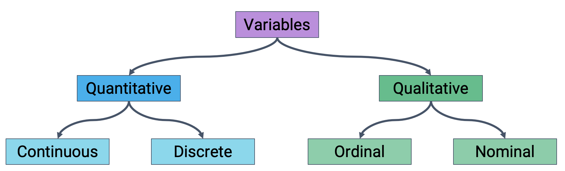### Primary and Foreign KeysLast time, we introduced `.merge` as the `pandas` method for joining multiple DataFrames together. In our discussion of joins, we touched on the idea of using a "key" to determine what rows should be merged from each table. Let's take a moment to examine this idea more closely.The **primary key** is the column or set of columns in a table that determine the values of the remaining columns. It can be thought of as the unique identifier for each individual row in the table. For example, a table of Data 100 students might use each student's Cal ID as the primary key. ```{python}#| echo: false#| vscode: {languageId: python}pd.DataFrame({"Cal ID":[3034619471, 3035619472, 3025619473, 3046789372], \"Name":["Oski", "Ollie", "Orrie", "Ollie"], \"Major":["Data Science", "Computer Science", "Data Science", "Economics"]})```The **foreign key** is the column or set of columns in a table that reference primary keys in other tables. Knowing a dataset's foreign keys can be useful when assigning the `left_on` and `right_on` parameters of `.merge`. In the table of office hour tickets below, `"Cal ID"` is a foreign key referencing the previous table.```{python}#| echo: false#| vscode: {languageId: python}pd.DataFrame({"OH Request":[1, 2, 3, 4], \"Cal ID":[3034619471, 3035619472, 3025619473, 3035619472], \"Question":["HW 2 Q1", "HW 2 Q3", "Lab 3 Q4", "HW 2 Q7"]})```## Granularity, Scope, and TemporalityAfter understanding the structure of the dataset, the next task is to determine what exactly the data represents. We'll do so by considering the data's granularity, scope, and temporality.The **granularity** of a dataset is what a single row represents. You can also think of it as the level of detail included in the data. To determine the data's granularity, ask: what does each row in the dataset represent? Fine-grained data contains a high level of detail, with a single row representing a small individual unit. For example, each record may represent one person. Coarse-grained data is encoded such that a single row represents a large individual unit – for example, each record may represent a group of people.The **scope** of a dataset is the subset of the population covered by the data. If we were investigating student performance in Data Science courses, a dataset with narrow scope might encompass all students enrolled in Data 100; a dataset with expansive scope might encompass all students in California. The **temporality** of a dataset describes the time period over which the data was collected. To fully understand the temporality of the data, it may be necessary to standardize timezones or inspect recurring time-based trends in the data (Do patterns recur in 24-hour patterns? Over the course of a month? Seasonally?).## FaithfulnessAt this stage in our data cleaning and EDA workflow, we've achieved quite a lot: we've identified how our data is structured, come to terms with what information it encodes, and gained insight as to how it was generated. Throughout this process, we should always recall the original intent of our work in Data Science – to use data to better understand and model the real world. To achieve this goal, we need to ensure that the data we use is faithful to reality; that is, that our data accurately captures the "real world."Data used in research or industry is often "messy" – there may be errors or inaccuracies that impact the faithfulness of the dataset. Signs that data may not be faithful include:* Unrealistic or "incorrect" values, such as negative counts, locations that don't exist, or dates set in the future* Violations of obvious dependencies, like an age that does not match a birthday* Clear signs that data was entered by hand, which can lead to spelling errors or fields that are incorrectly shifted* Signs of data falsification, such as fake email addresses or repeated use of the same names* Duplicated records or fields containing the same informationA common issue encountered with real-world datasets is that of missing data. One strategy to resolve this is to simply drop any records with missing values from the dataset. This does, however, introduce the risk of inducing biases – it is possible that the missing or corrupt records may be systemically related to some feature of interest in the data.Another method to address missing data is to perform **imputation**: infer the missing values using other data available in the dataset. There is a wide variety of imputation techniques that can be implemented; some of the most common are listed below.* Average imputation: replace missing values with the average value for that field* Hot deck imputation: replace missing values with some random value* Regression imputation: develop a model to predict missing values* Multiple imputation: replace missing values with multiple random valuesRegardless of the strategy used to deal with missing data, we should think carefully about *why* particular records or fields may be missing – this can help inform whether or not the absence of these values is signficant in some meaningful way.# EDA Demo: Tuberculosis in the United StatesNow, let's follow this data-cleaning and EDA workflow to see what can we say about the presence of Tuberculosis in the United States!We will examine the data included in the [original CDC article](https://www.cdc.gov/mmwr/volumes/71/wr/mm7112a1.htm?s_cid=mm7112a1_w#T1_down) published in 2021.## CSVs and Field NamesSuppose Table 1 was saved as a CSV file located in `data/cdc_tuberculosis.csv`.We can then explore the CSV (which is a text file, and does not contain binary-encoded data) in many ways:1. Using a text editor like emacs, vim, VSCode, etc.2. Opening the CSV directly in DataHub (read-only), Excel, Google Sheets, etc.3. The Python file object4. pandas, using `pd.read_csv()`1, 2. Let's start with the first two so we really solidify the idea of a CSV as **rectangular data (i.e., tabular data) stored as comma-separated values**.3. Next, let's try using the Python file object. Let's check out the first three lines:```{python}#| code-fold: false#| vscode: {languageId: python}withopen("data/cdc_tuberculosis.csv", "r") as f: i =0for row in f:print(row) i +=1if i >3:break```Whoa, why are there blank lines interspaced between the lines of the CSV?You may recall that all line breaks in text files are encoded as the special newline character `\n`. Python's `print()` prints each string (including the newline), and an additional newline on top of that.If you're curious, we can use the `repr()` function to return the raw string with all special characters:```{python}#| code-fold: false#| vscode: {languageId: python}withopen("data/cdc_tuberculosis.csv", "r") as f: i =0for row in f:print(repr(row)) # print raw strings i +=1if i >3:break```4. Finally, let's see the tried-and-true Data 100 approach: pandas.```{python}#| code-fold: false#| vscode: {languageId: python}tb_df = pd.read_csv("data/cdc_tuberculosis.csv")tb_df.head()```Wait, what's up with the "Unnamed" column names? And the first row, for that matter?Congratulations -- you're ready to wrangle your data. Because of how things are stored, we'll need to clean the data a bit to name our columns better.A reasonable first step is to identify the row with the right header. The `pd.read_csv()` function ([documentation](https://pandas.pydata.org/docs/reference/api/pandas.read_csv.html)) has the convenient `header` parameter:```{python}#| code-fold: false#| vscode: {languageId: python}tb_df = pd.read_csv("data/cdc_tuberculosis.csv", header=1) # row indextb_df.head(5)```Wait...but now we can't differentiate betwen the "Number of TB cases" and "TB incidence" year columns. pandas has tried to make our lives easier by automatically adding ".1" to the latter columns, but this doesn't help us as humans understand the data.We can do this manually with `df.rename()` ([documentation](https://pandas.pydata.org/docs/reference/api/pandas.DataFrame.rename.html?highlight=rename#pandas.DataFrame.rename)):```{python}#| code-fold: false#| vscode: {languageId: python}rename_dict = {'2019': 'TB cases 2019','2020': 'TB cases 2020','2021': 'TB cases 2021','2019.1': 'TB incidence 2019','2020.1': 'TB incidence 2020','2021.1': 'TB incidence 2021'}tb_df = tb_df.rename(columns=rename_dict)tb_df.head(5)```## Record GranularityYou might already be wondering: What's up with that first record?Row 0 is what we call a **rollup record**, or summary record. It's often useful when displaying tables to humans. The **granularity** of record 0 (Totals) vs the rest of the records (States) is different.Okay, EDA step two. How was the rollup record aggregated?Let's check if Total TB cases is the sum of all state TB cases. If we sum over all rows, we should get **2x** the total cases in each of our TB cases by year (why?).```{python}#| code-fold: false#| vscode: {languageId: python}tb_df.sum(axis=0)```Whoa, what's going on? Check out the column types:```{python}#| code-fold: false#| vscode: {languageId: python}tb_df.dtypes```Looks like those commas are causing all TB cases to be read as the `object` datatype, or **storage type** (close to the Python string datatype), so pandas is concatenating strings instead of adding integers.Fortunately `read_csv` also has a [`thousands` parameter](https://pandas.pydata.org/docs/reference/api/pandas.read_csv.html):```{python}#| code-fold: false#| vscode: {languageId: python}# improve readability: chaining method calls with outer parentheses/line breakstb_df = ( pd.read_csv("data/cdc_tuberculosis.csv", header=1, thousands=',') .rename(columns=rename_dict))tb_df.head(5)``````{python}#| code-fold: false#| vscode: {languageId: python}tb_df.sum()```The Total TB cases look right. Phew!Let's just look at the records with **state-level granularity**:```{python}#| code-fold: false#| vscode: {languageId: python}state_tb_df = tb_df[1:]state_tb_df.head(5)```## Gather More Data: CensusU.S. Census population estimates [source](https://www.census.gov/data/tables/time-series/demo/popest/2010s-state-total.html) (2019), [source](https://www.census.gov/data/tables/time-series/demo/popest/2020s-state-total.html) (2020-2021).Running the below cells cleans the data.There are a few new methods here:* `df.convert_dtypes()` ([documentation](https://pandas.pydata.org/docs/reference/api/pandas.DataFrame.convert_dtypes.html)) conveniently converts all float dtypes into ints and is out of scope for the class.* `df.drop_na()` ([documentation](https://pandas.pydata.org/docs/reference/api/pandas.DataFrame.dropna.html)) will be explained in more detail next time.```{python}#| code-fold: false#| vscode: {languageId: python}# 2010s census datacensus_2010s_df = pd.read_csv("data/nst-est2019-01.csv", header=3, thousands=",")census_2010s_df = ( census_2010s_df .reset_index() .drop(columns=["index", "Census", "Estimates Base"]) .rename(columns={"Unnamed: 0": "Geographic Area"}) .convert_dtypes() # "smart" converting of columns, use at your own risk .dropna() # we'll introduce this next time)census_2010s_df['Geographic Area'] = census_2010s_df['Geographic Area'].str.strip('.')# with pd.option_context('display.min_rows', 30): # shows more rows# display(census_2010s_df)census_2010s_df.head(5)```Occasionally, you will want to modify code that you have imported. To reimport those modifications you can either use the python importlib library:```pythonfrom importlib importreloadreload(utils)```or use iPython magic which will intelligently import code when files change:```python%load_ext autoreload%autoreload 2``````{python}#| code-fold: false#| vscode: {languageId: python}# census 2020s datacensus_2020s_df = pd.read_csv("data/NST-EST2022-POP.csv", header=3, thousands=",")census_2020s_df = ( census_2020s_df .reset_index() .drop(columns=["index", "Unnamed: 1"]) .rename(columns={"Unnamed: 0": "Geographic Area"}) .convert_dtypes() # "smart" converting of columns, use at your own risk .dropna() # we'll introduce this next time)census_2020s_df['Geographic Area'] = census_2020s_df['Geographic Area'].str.strip('.')census_2020s_df.head(5)```## Joining Data on Primary KeysTime to `merge`! Here we use the DataFrame method `df1.merge(right=df2, ...)` on DataFrame `df1` ([documentation](https://pandas.pydata.org/docs/reference/api/pandas.DataFrame.merge.html)). Contrast this with the function `pd.merge(left=df1, right=df2, ...)` ([documentation](https://pandas.pydata.org/docs/reference/api/pandas.merge.html?highlight=pandas%20merge#pandas.merge)). Feel free to use either.```{python}#| code-fold: false#| vscode: {languageId: python}# merge TB dataframe with two US census dataframestb_census_df = ( tb_df .merge(right=census_2010s_df, left_on="U.S. jurisdiction", right_on="Geographic Area") .merge(right=census_2020s_df, left_on="U.S. jurisdiction", right_on="Geographic Area"))tb_census_df.head(5)```This is a little unwieldy. We could either drop the unneeded columns now, or just merge on smaller census DataFrames. Let's do the latter.```{python}#| code-fold: false#| vscode: {languageId: python}# try merging again, but cleaner this timetb_census_df = ( tb_df .merge(right=census_2010s_df[["Geographic Area", "2019"]], left_on="U.S. jurisdiction", right_on="Geographic Area") .drop(columns="Geographic Area") .merge(right=census_2020s_df[["Geographic Area", "2020", "2021"]], left_on="U.S. jurisdiction", right_on="Geographic Area") .drop(columns="Geographic Area"))tb_census_df.head(5)```## Reproducing Data: Compute IncidenceLet's recompute incidence to make sure we know where the original CDC numbers came from.From the [CDC report](https://www.cdc.gov/mmwr/volumes/71/wr/mm7112a1.htm?s_cid=mm7112a1_w#T1_down): TB incidence is computed as “Cases per 100,000 persons using mid-year population estimates from the U.S. Census Bureau.”If we define a group as 100,000 people, then we can compute the TB incidence for a given state population as$$\text{TB incidence} = \frac{\text{TB cases in population}}{\text{groups in population}} = \frac{\text{TB cases in population}}{\text{population}/100000} $$$$= \frac{\text{TB cases in population}}{\text{population}} \times 100000$$Let's try this for 2019:```{python}#| code-fold: false#| vscode: {languageId: python}tb_census_df["recompute incidence 2019"] = tb_census_df["TB cases 2019"]/tb_census_df["2019"]*100000tb_census_df.head(5)```Awesome!!!Let's use a for-loop and Python format strings to compute TB incidence for all years. Python f-strings are just used for the purposes of this demo, but they're handy to know when you explore data beyond this course ([Python documentation](https://docs.python.org/3/tutorial/inputoutput.html)).```{python}#| code-fold: false#| vscode: {languageId: python}# recompute incidence for all yearsfor year in [2019, 2020, 2021]: tb_census_df[f"recompute incidence {year}"] = tb_census_df[f"TB cases {year}"]/tb_census_df[f"{year}"]*100000tb_census_df.head(5)```These numbers look pretty close!!! There are a few errors in the hundredths place, particularly in 2021. It may be useful to further explore reasons behind this discrepancy. ```{python}#| code-fold: false#| vscode: {languageId: python}tb_census_df.describe()```## Bonus EDA: Reproducing the reported statistic**How do we reproduce that reported statistic in the original [CDC report](https://www.cdc.gov/mmwr/volumes/71/wr/mm7112a1.htm?s_cid=mm7112a1_w)?**> Reported TB incidence (cases per 100,000 persons) increased **9.4%**, from **2.2** during 2020 to **2.4** during 2021 but was lower than incidence during 2019 (2.7). Increases occurred among both U.S.-born and non–U.S.-born persons.This is TB incidence computed across the entire U.S. population! How do we reproduce this* We need to reproduce the "Total" TB incidences in our rolled record.* But our current `tb_census_df` only has 51 entries (50 states plus Washington, D.C.). There is no rolled record.* What happened...?Let's get exploring!Before we keep exploring, we'll set all indexes to more meaningful values, instead of just numbers that pertained to some row at some point. This will make our cleaning slightly easier.```{python}#| code-fold: false#| vscode: {languageId: python}tb_df = tb_df.set_index("U.S. jurisdiction")tb_df.head(5)``````{python}#| code-fold: false#| vscode: {languageId: python}census_2010s_df = census_2010s_df.set_index("Geographic Area")census_2010s_df.head(5)``````{python}#| code-fold: false#| vscode: {languageId: python}census_2020s_df = census_2020s_df.set_index("Geographic Area")census_2020s_df.head(5)```It turns out that our merge above only kept state records, even though our original `tb_df` had the "Total" rolled record:```{python}#| code-fold: false#| vscode: {languageId: python}tb_df.head()```Recall that merge by default does an **inner** merge by default, meaning that it only preserves keys that are present in **both** DataFrames.The rolled records in our census dataframes have different `Geographic Area` fields, which was the key we merged on:```{python}#| code-fold: false#| vscode: {languageId: python}census_2010s_df.head(5)```The Census DataFrame has several rolled records. The aggregate record we are looking for actually has the Geographic Area named "United States".One straightforward way to get the right merge is to rename the value itself. Because we now have the Geographic Area index, we'll use `df.rename()` ([documentation](https://pandas.pydata.org/docs/reference/api/pandas.DataFrame.rename.html)):```{python}#| code-fold: false#| vscode: {languageId: python}# rename rolled record for 2010scensus_2010s_df.rename(index={'United States':'Total'}, inplace=True)census_2010s_df.head(5)``````{python}#| code-fold: false#| vscode: {languageId: python}# same, but for 2020s rename rolled recordcensus_2020s_df.rename(index={'United States':'Total'}, inplace=True)census_2020s_df.head(5)```<br/>Next let's rerun our merge. Note the different chaining, because we are now merging on indexes (`df.merge()`[documentation](https://pandas.pydata.org/docs/reference/api/pandas.DataFrame.merge.html)).```{python}#| code-fold: false#| vscode: {languageId: python}tb_census_df = ( tb_df .merge(right=census_2010s_df[["2019"]], left_index=True, right_index=True) .merge(right=census_2020s_df[["2020", "2021"]], left_index=True, right_index=True))tb_census_df.head(5)```<br/>Finally, let's recompute our incidences:```{python}#| code-fold: false#| vscode: {languageId: python}# recompute incidence for all yearsfor year in [2019, 2020, 2021]: tb_census_df[f"recompute incidence {year}"] = tb_census_df[f"TB cases {year}"]/tb_census_df[f"{year}"]*100000tb_census_df.head(5)```We reproduced the total U.S. incidences correctly!We're almost there. Let's revisit the quote:> Reported TB incidence (cases per 100,000 persons) increased **9.4%**, from **2.2** during 2020 to **2.4** during 2021 but was lower than incidence during 2019 (2.7). Increases occurred among both U.S.-born and non–U.S.-born persons.Recall that percent change from $A$ to $B$ is computed as$\text{percent change} = \frac{B - A}{A} \times 100$.```{python}#| code-fold: false#| tags: []#| vscode: {languageId: python}incidence_2020 = tb_census_df.loc['Total', 'recompute incidence 2020']incidence_2020``````{python}#| code-fold: false#| tags: []#| vscode: {languageId: python}incidence_2021 = tb_census_df.loc['Total', 'recompute incidence 2021']incidence_2021``````{python}#| code-fold: false#| tags: []#| vscode: {languageId: python}difference = (incidence_2021 - incidence_2020)/incidence_2020 *100difference```
