2 Pandas I

Learning Outcomes

Build familiarity with basic pandas syntax
Learn key data structures: DataFrames, Series, and Indices
Understand methods for extracting data: .loc, .iloc, and [ ]

In this sequence of lectures, we will dive right into things by having you explore and manipulate real-world data. To do so, we’ll introduce pandas, a popular Python library for interacting with tabular data.

2.1 Tabular Data

Data scientists work with data stored in a variety of formats. The primary focus of this class is in understanding tabular data –– data that is stored in a table.

Tabular data is one of the most common systems that data scientists use to organize data. This is in large part due to the simplicity and flexibility of tables. Tables allow us to represent each observation, or instance of collecting data from an individual, as its own row. We can record distinct characteristics, or features, of each observation in separate columns.

To see this in action, we’ll explore the elections dataset, which stores information about political candidates who ran for president of the United States in various years.

Code

import pandas as pd
pd.read_csv("data/elections.csv")

	Year	Candidate	Party	Popular vote	Result	%
0	1824	Andrew Jackson	Democratic-Republican	151271	loss	57.210122
1	1824	John Quincy Adams	Democratic-Republican	113142	win	42.789878
2	1828	Andrew Jackson	Democratic	642806	win	56.203927
3	1828	John Quincy Adams	National Republican	500897	loss	43.796073
4	1832	Andrew Jackson	Democratic	702735	win	54.574789
...	...	...	...	...	...	...
177	2016	Jill Stein	Green	1457226	loss	1.073699
178	2020	Joseph Biden	Democratic	81268924	win	51.311515
179	2020	Donald Trump	Republican	74216154	loss	46.858542
180	2020	Jo Jorgensen	Libertarian	1865724	loss	1.177979
181	2020	Howard Hawkins	Green	405035	loss	0.255731

182 rows × 6 columns

In the elections dataset, each row represents one instance of a candidate running for president in a particular year. For example, the first row represents Andrew Jackson running for president in the year 1824. Each column represents one characteristic piece of information about each presidential candidate. For example, the column named “Result” stores whether or not the candidate won the electon.

Your work in Data 8 helped you grow very familiar with using and interpreting data stored in a tabular format. Back then, you used the Table class of the datascience library, a special programming library specifically for Data 8 students.

In Data 100, we will be working with the programming library pandas, which is generally accepted in the data science community as the industry- and academia-standard tool for manipulating tabular data (as well as the inspiration for Petey, our panda bear mascot).

2.2 DataFrames, Series, and Indices

To begin our studies in pandas, we must first import the library into our Python environment. This will allow us to use pandas data structures and methods in our code.

# `pd` is the conventional alias for Pandas, as `np` is for NumPy
import pandas as pd

There are three fundamental data structures in pandas:

Series: 1D labeled array data; best thought of as columnar data
DataFrame: 2D tabular data with rows and columns
Index: A sequence of row/column labels

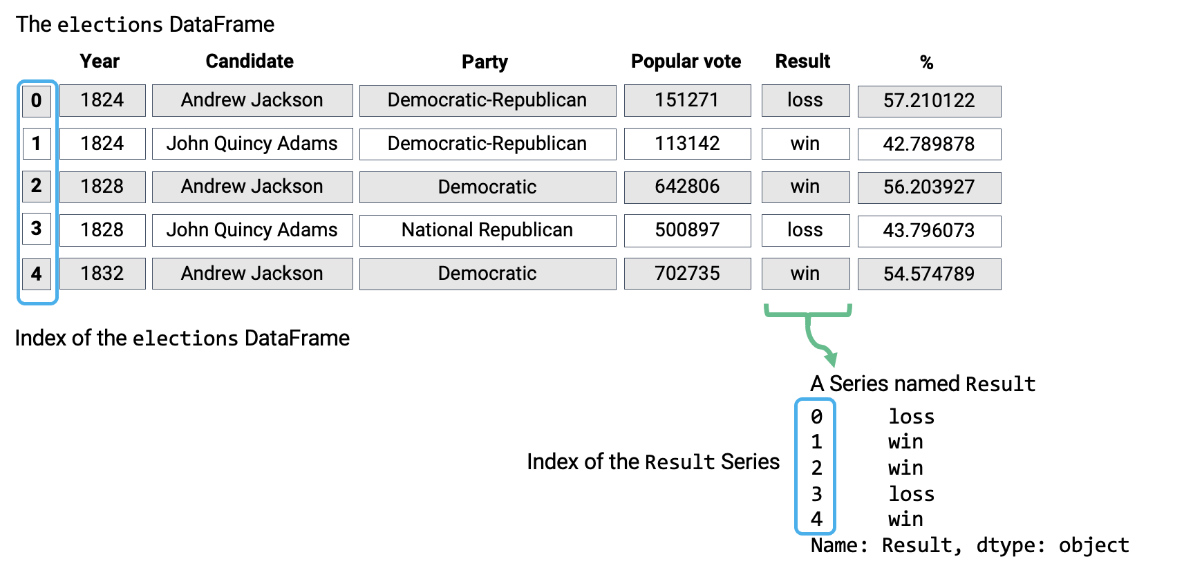
DataFrames, Series, and Indices can be represented visually in the following diagram, which considers the first few rows of the elections dataset.

Notice how the DataFrame is a two-dimensional object – it contains both rows and columns. The Series above is a singular column of this DataFrame, namely, the Result column. Both contain an Index, or a shared list of row labels (here, the integers from 0 to 4, inclusive).

2.2.1 Series

A Series represents a column of a DataFrame; more generally, it can be any 1-dimensional array-like object containing values of the same type with associated data labels, called its index. In the cell below, we create a Series named s.

s = pd.Series([-1, 10, 2])
s

0    -1
1    10
2     2
dtype: int64

s.values # Data contained within the Series

array([-1, 10,  2])

s.index # The Index of the Series

RangeIndex(start=0, stop=3, step=1)

By default, the Index of a Series is a sequential list of integers beginning from 0. Optionally, a manually-specified list of desired indices can be passed to the index argument.

s = pd.Series([-1, 10, 2], index = ["a", "b", "c"])
s

a    -1
b    10
c     2
dtype: int64

Indices can also be changed after initialization.

s.index = ["first", "second", "third"]
s

first     -1
second    10
third      2
dtype: int64

2.2.1.1 Selection in Series

Much like when working with NumPy arrays, we can select a single value or a set of values from a Series. There are 3 primary methods of selecting data.

A single index label
A list of index labels
A filtering condition

To demonstrate this, let’s define the Series ser.

ser = pd.Series([4, -2, 0, 6], index = ["a", "b", "c", "d"])
ser

a    4
b   -2
c    0
d    6
dtype: int64

2.2.1.1.1 A Single Index Label

ser["a"] # We return the value stored at the Index label "a"

2.2.1.1.2 A List of Index Labels

ser[["a", "c"]] # We return a *Series* of the values stored at labels "a" and "c"

a    4
c    0
dtype: int64

2.2.1.1.3 A Filtering Condition

Perhaps the most interesting (and useful) method of selecting data from a Series is with a filtering condition.

First, we apply a boolean condition to the Series. This create a new Series of boolean values.

ser > 0 # Filter condition: select all elements greater than 0

a     True
b    False
c    False
d     True
dtype: bool

We then use this boolean condition to index into our original Series. pandas will select only the entries in the original Series that satisfy the condition.

ser[ser > 0]

a    4
d    6
dtype: int64

2.2.2 DataFrames

In Data 8, you represented tabular data using the Table class of the datascience library. In Data 100, we’ll be using the DataFrame class of the pandas library.

With our new understanding of pandas in hand, let’s return to the elections dataset from before. Now, we recognize that it is represented as a pandas DataFrame.

import pandas as pd

elections = pd.read_csv("data/elections.csv")
elections

	Year	Candidate	Party	Popular vote	Result	%
0	1824	Andrew Jackson	Democratic-Republican	151271	loss	57.210122
1	1824	John Quincy Adams	Democratic-Republican	113142	win	42.789878
2	1828	Andrew Jackson	Democratic	642806	win	56.203927
3	1828	John Quincy Adams	National Republican	500897	loss	43.796073
4	1832	Andrew Jackson	Democratic	702735	win	54.574789
...	...	...	...	...	...	...
177	2016	Jill Stein	Green	1457226	loss	1.073699
178	2020	Joseph Biden	Democratic	81268924	win	51.311515
179	2020	Donald Trump	Republican	74216154	loss	46.858542
180	2020	Jo Jorgensen	Libertarian	1865724	loss	1.177979
181	2020	Howard Hawkins	Green	405035	loss	0.255731

182 rows × 6 columns

Let’s dissect the code above.

We first import the pandas library into our Python environment, using the alias pd.
import pandas as pd
There are a number of ways to read data into a DataFrame. In Data 100, our datasets are typically stored in a CSV (comma-seperated values) file format. We can import a CSV file into a DataFrame by passing the data path as an argument to the following pandas function.
pd.read_csv("data/elections.csv")

This code stores our DataFrame object in the elections variable. We see that our elections DataFrame has 182 rows and 6 columns (Year, Candidate, Party, Popular Vote, Result, %). Each row represents a single record – in our example, a presedential candidate from some particular year. Each column represents a single attribute, or feature of the record.

In the example above, we constructed a DataFrame object using data from a CSV file. As we’ll explore in the next section, we can also create a DataFrame with data of our own.

2.2.2.1 Creating a DataFrame

There are many ways to create a DataFrame. Here, we will cover the most popular approaches.

Using a list and column names
From a dictionary
From a Series

2.2.2.1.1 Using a List and Column Names

Consider the following examples. The first code cell creates a DataFrame with a single column Numbers. The second creates a DataFrame with the columns Numbers and Description. Notice how a 2D list of values is required to initialize the second DataFrame – each nested list represents a single row of data.

df_list_1 = pd.DataFrame([1, 2, 3], columns=["Numbers"])
df_list_1

	Numbers
0	1
1	2
2	3

df_list_2 = pd.DataFrame([[1, "one"], [2, "two"]], columns = ["Number", "Description"])
df_list_2

	Number	Description
0	1	one
1	2	two

2.2.2.1.2 From a Dictionary

A second (and more common) way to create a DataFrame is with a dictionary. The dictionary keys represent the column names, and the dictionary values represent the column values.

df_dict = pd.DataFrame({"Fruit": ["Strawberry", "Orange"], "Price": [5.49, 3.99]})
df_dict

	Fruit	Price
0	Strawberry	5.49
1	Orange	3.99

2.2.2.1.3 From a Series

Earlier, we noted that a Series is usually thought of as a column in a DataFrame. It follows then, that a DataFrame is equivalent to a collection of Series, which all share the same index.

In fact, we can initialize a DataFrame by merging two or more Series.

# Notice how our indices, or row labels, are the same

s_a = pd.Series(["a1", "a2", "a3"], index = ["r1", "r2", "r3"])
s_b = pd.Series(["b1", "b2", "b3"], index = ["r1", "r2", "r3"])

pd.DataFrame({"A-column": s_a, "B-column": s_b})

	A-column	B-column
r1	a1	b1
r2	a2	b2
r3	a3	b3

2.2.3 Indices

The major takeaway: we can think of a DataFrame as a collection of Series that all share the same Index.

On a more technical note, an Index doesn’t have to be an integer, nor does it have to be unique. For example, we can set the index of the elections Dataframe to be the name of presidential candidates.

# This sets the index to be the "Candidate" column
elections.set_index("Candidate", inplace=True)
elections.index

Index(['Andrew Jackson', 'John Quincy Adams', 'Andrew Jackson',
       'John Quincy Adams', 'Andrew Jackson', 'Henry Clay', 'William Wirt',
       'Hugh Lawson White', 'Martin Van Buren', 'William Henry Harrison',
       ...
       'Darrell Castle', 'Donald Trump', 'Evan McMullin', 'Gary Johnson',
       'Hillary Clinton', 'Jill Stein', 'Joseph Biden', 'Donald Trump',
       'Jo Jorgensen', 'Howard Hawkins'],
      dtype='object', name='Candidate', length=182)

And, if we’d like, we can revert the index back to the default list of integers.

# This resets the index to be the default list of integers
elections.reset_index(inplace=True) 
elections.index

RangeIndex(start=0, stop=182, step=1)

2.3 Slicing in DataFrames

Now that we’ve learned how to create DataFrames, let’s dive more deeply into their capabilities.

The API (application programming interface) for the DataFrame class is enormous. In this section, we’ll discuss several methods of the DataFrame API that allow us to extract subsets of data.

The simplest way to manipulate a DataFrame is to extract a subset of rows and columns, known as slicing. We will do so with four primary methods of the DataFrame class:

.head and .tail
.loc
.iloc
[]

2.3.1 Extracting data with `.head` and `.tail`

The simplest scenario in which we want to extract data is when we simply want to select the first or last few rows of the DataFrame.

To extract the first n rows of a DataFrame df, we use the syntax df.head(n).

# Extract the first 5 rows of the DataFrame
elections.head(5)

	Candidate	Year	Party	Popular vote	Result	%
0	Andrew Jackson	1824	Democratic-Republican	151271	loss	57.210122
1	John Quincy Adams	1824	Democratic-Republican	113142	win	42.789878
2	Andrew Jackson	1828	Democratic	642806	win	56.203927
3	John Quincy Adams	1828	National Republican	500897	loss	43.796073
4	Andrew Jackson	1832	Democratic	702735	win	54.574789

Similarly, calling df.tail(n) allows us to extract the last n rows of the DataFrame.

# Extract the last 5 rows of the DataFrame
elections.tail(5)

	Candidate	Year	Party	Popular vote	Result	%
177	Jill Stein	2016	Green	1457226	loss	1.073699
178	Joseph Biden	2020	Democratic	81268924	win	51.311515
179	Donald Trump	2020	Republican	74216154	loss	46.858542
180	Jo Jorgensen	2020	Libertarian	1865724	loss	1.177979
181	Howard Hawkins	2020	Green	405035	loss	0.255731

2.3.2 Indexing with .loc

The .loc operator selects rows and columns in a DataFrame by their row and column label(s), respectively. The row labels (commonly referred to as the indices) are the bold text on the far left of a DataFrame, while the column labels are the column names found at the top of a DataFrame.

To grab data with .loc, we must specify the row and column label(s) where the data exists. The row labels are the first argument to the .loc function; the column labels are the second. For example, we can select the the row labeled 0 and the column labeled Candidate from the elections DataFrame.

elections.loc[0, 'Candidate']

'Andrew Jackson'

To select multiple rows and columns, we can use Python slice notation. Here, we select the rows from labels 0 to 3 and the columns from labels "Year" to "Popular vote".

elections.loc[0:3, 'Year':'Popular vote']

	Year	Party	Popular vote
0	1824	Democratic-Republican	151271
1	1824	Democratic-Republican	113142
2	1828	Democratic	642806
3	1828	National Republican	500897

Suppose that instead, we wanted every column value for the first four rows in the elections DataFrame. The shorthand : is useful for this.

elections.loc[0:3, :]

	Candidate	Year	Party	Popular vote	Result	%
0	Andrew Jackson	1824	Democratic-Republican	151271	loss	57.210122
1	John Quincy Adams	1824	Democratic-Republican	113142	win	42.789878
2	Andrew Jackson	1828	Democratic	642806	win	56.203927
3	John Quincy Adams	1828	National Republican	500897	loss	43.796073

There are a couple of things we should note. Firstly, unlike conventional Python, Pandas allows us to slice string values (in our example, the column labels). Secondly, slicing with .loc is inclusive. Notice how our resulting DataFrame includes every row and column between and including the slice labels we specified.

Equivalently, we can use a list to obtain multiple rows and columns in our elections DataFrame.

elections.loc[[0, 1, 2, 3], ['Year', 'Candidate', 'Party', 'Popular vote']]

	Year	Candidate	Party	Popular vote
0	1824	Andrew Jackson	Democratic-Republican	151271
1	1824	John Quincy Adams	Democratic-Republican	113142
2	1828	Andrew Jackson	Democratic	642806
3	1828	John Quincy Adams	National Republican	500897

Lastly, we can interchange list and slicing notation.

elections.loc[[0, 1, 2, 3], :]

	Candidate	Year	Party	Popular vote	Result	%
0	Andrew Jackson	1824	Democratic-Republican	151271	loss	57.210122
1	John Quincy Adams	1824	Democratic-Republican	113142	win	42.789878
2	Andrew Jackson	1828	Democratic	642806	win	56.203927
3	John Quincy Adams	1828	National Republican	500897	loss	43.796073

2.3.3 Indexing with .iloc

Slicing with .iloc works similarily to .loc, however, .iloc uses the index positions of rows and columns rather the labels (think to yourself: loc uses labels; iloc uses indices). The arguments to the .iloc function also behave similarly -– single values, lists, indices, and any combination of these are permitted.

Let’s begin reproducing our results from above. We’ll begin by selecting for the first presidential candidate in our elections DataFrame:

# elections.loc[0, "Candidate"] - Previous approach
elections.iloc[0, 1]

Notice how the first argument to both .loc and .iloc are the same. This is because the row with a label of 0 is conveniently in the 0^th index (equivalently, the first position) of the elections DataFrame. Generally, this is true of any DataFrame where the row labels are incremented in ascending order from 0.

However, when we select the first four rows and columns using .iloc, we notice something.

# elections.loc[0:3, 'Year':'Popular vote'] - Previous approach
elections.iloc[0:4, 0:4]

	Candidate	Year	Party	Popular vote
0	Andrew Jackson	1824	Democratic-Republican	151271
1	John Quincy Adams	1824	Democratic-Republican	113142
2	Andrew Jackson	1828	Democratic	642806
3	John Quincy Adams	1828	National Republican	500897

Slicing is no longer inclusive in .iloc -– it’s exclusive. In other words, the right-end of a slice is not included when using .iloc. This is one of the subtleties of pandas syntax; you will get used to it with practice.

List behavior works just as expected.

#elections.loc[[0, 1, 2, 3], ['Year', 'Candidate', 'Party', 'Popular vote']] - Previous Approach
elections.iloc[[0, 1, 2, 3], [0, 1, 2, 3]]

	Candidate	Year	Party	Popular vote
0	Andrew Jackson	1824	Democratic-Republican	151271
1	John Quincy Adams	1824	Democratic-Republican	113142
2	Andrew Jackson	1828	Democratic	642806
3	John Quincy Adams	1828	National Republican	500897

This discussion begs the question: when should we use .loc vs .iloc? In most cases, .loc is generally safer to use. You can imagine .iloc may return incorrect values when applied to a dataset where the ordering of data can change.

2.3.4 Indexing with []

The [] selection operator is the most baffling of all, yet the most commonly used. It only takes a single argument, which may be one of the following:

A slice of row numbers
A list of column labels
A single column label

That is, [] is context dependent. Let’s see some examples.

2.3.4.1 A slice of row numbers

Say we wanted the first four rows of our elections DataFrame.

elections[0:4]

	Candidate	Year	Party	Popular vote	Result	%
0	Andrew Jackson	1824	Democratic-Republican	151271	loss	57.210122
1	John Quincy Adams	1824	Democratic-Republican	113142	win	42.789878
2	Andrew Jackson	1828	Democratic	642806	win	56.203927
3	John Quincy Adams	1828	National Republican	500897	loss	43.796073

2.3.4.2 A list of column labels

Suppose we now want the first four columns.

elections[["Year", "Candidate", "Party", "Popular vote"]]

	Year	Candidate	Party	Popular vote
0	1824	Andrew Jackson	Democratic-Republican	151271
1	1824	John Quincy Adams	Democratic-Republican	113142
2	1828	Andrew Jackson	Democratic	642806
3	1828	John Quincy Adams	National Republican	500897
4	1832	Andrew Jackson	Democratic	702735
...	...	...	...	...
177	2016	Jill Stein	Green	1457226
178	2020	Joseph Biden	Democratic	81268924
179	2020	Donald Trump	Republican	74216154
180	2020	Jo Jorgensen	Libertarian	1865724
181	2020	Howard Hawkins	Green	405035

182 rows × 4 columns

2.3.4.3 A single column label

Lastly, [ ] allows us to extract only the Candidate column.

elections["Candidate"]

0         Andrew Jackson
1      John Quincy Adams
2         Andrew Jackson
3      John Quincy Adams
4         Andrew Jackson
             ...        
177           Jill Stein
178         Joseph Biden
179         Donald Trump
180         Jo Jorgensen
181       Howard Hawkins
Name: Candidate, Length: 182, dtype: object

The output is a Series! In this course, we’ll become very comfortable with [], especially for selecting columns. In practice, [] is much more common than .loc.

2.4 Parting Note

The pandas library is enormous and contains many useful functions. Here is a link to documentation. We certainly don’t expect you to memorize each and every method of the library.

The introductory Data 100 pandas lectures will provide a high-level view of the key data structures and methods that will form the foundation of your pandas knowledge. A goal of this course is to help you build your familiarity with the real-world programming practice of…Googling! Answers to your questions can be found in documentation, Stack Overflow, etc. Being able to search for, read, and implement documentation is an important life skill for any data scientist.

With that, let’s move on to Pandas II.

2.1 Tabular Data

2.2 DataFrames, Series, and Indices

2.2.1 Series

2.2.1.1 Selection in Series

2.2.1.1.1 A Single Index Label

2.2.1.1.2 A List of Index Labels

2.2.1.1.3 A Filtering Condition

2.2.2 DataFrames

2.2.2.1 Creating a DataFrame

2.2.2.1.1 Using a List and Column Names

2.2.2.1.2 From a Dictionary

2.2.2.1.3 From a Series

2.2.3 Indices

2.3 Slicing in DataFrames

2.3.1 Extracting data with .head and .tail

2.3.2 Indexing with .loc

2.3.3 Indexing with .iloc

2.3.4 Indexing with []

2.3.4.1 A slice of row numbers

2.3.4.2 A list of column labels

2.3.4.3 A single column label

2.4 Parting Note

2.3.1 Extracting data with `.head` and `.tail`