Extract data from a DataFrame using conditional selection
Recognize situations where aggregation is useful and identify the correct technique for performing an aggregation
Last time, we introduced the pandas library as a toolkit for processing data. We learned the DataFrame and Series data structures, familiarized ourselves with the basic syntax for manipulating tabular data, and began writing our first lines of pandas code.
In this lecture, we’ll start to dive into some advanced pandas syntax. You may find it helpful to follow along with a notebook of your own as we walk through these new pieces of code.
We’ll start by loading the babynames dataset.
Code
# This code pulls census data and loads it into a DataFrame# We won't cover it explicitly in this class, but you are welcome to explore it on your ownimport pandas as pdimport numpy as npimport urllib.requestimport os.pathimport zipfiledata_url ="https://www.ssa.gov/oact/babynames/state/namesbystate.zip"local_filename ="babynamesbystate.zip"ifnot os.path.exists(local_filename): # if the data exists don't download againwith urllib.request.urlopen(data_url) as resp, open(local_filename, 'wb') as f: f.write(resp.read())zf = zipfile.ZipFile(local_filename, 'r')ca_name ='CA.TXT'field_names = ['State', 'Sex', 'Year', 'Name', 'Count']with zf.open(ca_name) as fh: babynames = pd.read_csv(fh, header=None, names=field_names)babynames.head()
State
Sex
Year
Name
Count
0
CA
F
1910
Mary
295
1
CA
F
1910
Helen
239
2
CA
F
1910
Dorothy
220
3
CA
F
1910
Margaret
163
4
CA
F
1910
Frances
134
3.1 Conditional Selection
Conditional selection allows us to select a subset of rows in a DataFrame if they follow some specified condition.
To understand how to use conditional selection, we must look at another possible input of the .loc and [] methods – a boolean array, which is simply an array or Series where each element is either True or False. This boolean array must have a length equal to the number of rows in the DataFrame. It will return all rows that correspond to a value of True in the array. We used a very similar technique when performing conditional extraction from a Series in the last lecture.
To see this in action, let’s select all even-indexed rows in the first 10 rows of our DataFrame.
# Ask yourself: why is :9 is the correct slice to select the first 10 rows?babynames_first_10_rows = babynames.loc[:9, :]# Notice how we have exactly 10 elements in our boolean array argumentbabynames_first_10_rows[[True, False, True, False, True, False, True, False, True, False]]
These techniques worked well in this example, but you can imagine how tedious it might be to list out Trues and Falses for every row in a larger DataFrame. To make things easier, we can instead provide a logical condition as an input to .loc or [] that returns a boolean array with the necessary length.
For example, to return all names associated with F sex:
# First, use a logical condition to generate a boolean arraylogical_operator = (babynames["Sex"] =="F")# Then, use this boolean array to filter the DataFramebabynames[logical_operator].head()
State
Sex
Year
Name
Count
0
CA
F
1910
Mary
295
1
CA
F
1910
Helen
239
2
CA
F
1910
Dorothy
220
3
CA
F
1910
Margaret
163
4
CA
F
1910
Frances
134
Recall from the previous lecture that .head() will return only the first few rows in the DataFrame. In reality, babynames[logical operator] contains as many rows as there are entries in the original babynamesDataFrame with sex "F".
Here, logical_operator evaluates to a Series of boolean values with length 400762.
Code
print("There are a total of {} values in 'logical_operator'".format(len(logical_operator)))
There are a total of 400762 values in 'logical_operator'
Rows starting at row 0 and ending at row 235790 evaluate to True and are thus returned in the DataFrame. Rows from 235791 onwards evaluate to False and are omitted from the output.
Code
print("The 0th item in this 'logical_operator' is: {}".format(logical_operator.iloc[0]))print("The 235790th item in this 'logical_operator' is: {}".format(logical_operator.iloc[235790]))print("The 235791th item in this 'logical_operator' is: {}".format(logical_operator.iloc[235791]))
The 0th item in this 'logical_operator' is: True
The 235790th item in this 'logical_operator' is: True
The 235791th item in this 'logical_operator' is: False
Passing a Series as an argument to babynames[] has the same affect as using a boolean array. In fact, the [] selection operator can take a boolean Series, array, and list as arguments. These three are used interchangeably thoughout the course.
We can also use .loc to achieve similar results.
babynames.loc[babynames["Sex"] =="F"].head()
State
Sex
Year
Name
Count
0
CA
F
1910
Mary
295
1
CA
F
1910
Helen
239
2
CA
F
1910
Dorothy
220
3
CA
F
1910
Margaret
163
4
CA
F
1910
Frances
134
Boolean conditions can be combined using various bitwise operators that allow us to filter results by multiple conditions.
Symbol
Usage
Meaning
~
~p
Returns negation of p
|
p | q
p OR q
&
p & q
p AND q
^
p ^ q
p XOR q (exclusive or)
When combining multiple conditions with logical operators, we surround each individual condition with a set of parenthesis (). This imposes an order of operations on pandas evaluating your logic, and can avoid code erroring.
For example, if we want to return data on all names with sex "F" born before the 21st century, we can write:
Boolean array selection is a useful tool, but can lead to overly verbose code for complex conditions. In the example below, our boolean condition is long enough to extend for several lines of code.
# Note: The parentheses surrounding the code make it possible to break the code on to multiple lines for readability( babynames[(babynames["Name"] =="Bella") | (babynames["Name"] =="Alex") | (babynames["Name"] =="Ani") | (babynames["Name"] =="Lisa")]).head()
State
Sex
Year
Name
Count
6289
CA
F
1923
Bella
5
7512
CA
F
1925
Bella
8
12368
CA
F
1932
Lisa
5
14741
CA
F
1936
Lisa
8
17084
CA
F
1939
Lisa
5
Fortunately, pandas provides many alternative methods for constructing boolean filters.
The .isin function is one such example. This method evaluates if the values in a Series are contained in a different sequence (list, array, or Series) of values. In the cell below, we achieve equivalent result to the DataFrame above with far more concise code.
The function str.startswith can be used to define a filter based on string values in a Series object. It checks to see if string values in a Series start with a particular character.
# Find the names that begin with the letter "N"babynames[babynames["Name"].str.startswith("N")].head()
State
Sex
Year
Name
Count
76
CA
F
1910
Norma
23
83
CA
F
1910
Nellie
20
127
CA
F
1910
Nina
11
198
CA
F
1910
Nora
6
310
CA
F
1911
Nellie
23
3.2 Adding, Removing, and Modifying Columns
In many data science tasks, we may need to change the columns contained in our DataFrame in some way. Fortunately, the syntax to do so is fairly straightforward.
To add a new column to a DataFrame, we use a syntax similar to that used when accessing an existing column. Specify the name of the new column by writing df["column"], then assign this to a Series or array containing the values that will populate this column.
# Create a Series of the length of each name. We'll discuss `str` methods next week.babyname_lengths = babynames["Name"].str.len()# Add a column named "name_lengths" that includes the length of each namebabynames["name_lengths"] = babyname_lengthsbabynames.head(5)
State
Sex
Year
Name
Count
name_lengths
0
CA
F
1910
Mary
295
4
1
CA
F
1910
Helen
239
5
2
CA
F
1910
Dorothy
220
7
3
CA
F
1910
Margaret
163
8
4
CA
F
1910
Frances
134
7
If we need to later modify an existing column, we can do so by referencing this column again with the syntax df["column"], then re-assigning it to a new Series or array.
# Modify the “name_lengths” column to be one less than its original valuebabynames["name_lengths"] = babynames["name_lengths"]-1babynames.head()
State
Sex
Year
Name
Count
name_lengths
0
CA
F
1910
Mary
295
3
1
CA
F
1910
Helen
239
4
2
CA
F
1910
Dorothy
220
6
3
CA
F
1910
Margaret
163
7
4
CA
F
1910
Frances
134
6
We can rename a column using the .rename() method. .rename() takes in a dictionary that maps old column names to their new ones.
# Rename “name_lengths” to “Length”babynames = babynames.rename(columns={"name_lengths":"Length"})babynames.head()
State
Sex
Year
Name
Count
Length
0
CA
F
1910
Mary
295
3
1
CA
F
1910
Helen
239
4
2
CA
F
1910
Dorothy
220
6
3
CA
F
1910
Margaret
163
7
4
CA
F
1910
Frances
134
6
If we want to remove a column or row of a DataFrame, we can call the .drop method. Use the axis parameter to specify whether a column or row should be dropped. Unless otherwise specified, pandas will assume that we are dropping a row by default.
# Drop our new "Length" column from the DataFramebabynames = babynames.drop("Length", axis="columns")babynames.head(5)
State
Sex
Year
Name
Count
0
CA
F
1910
Mary
295
1
CA
F
1910
Helen
239
2
CA
F
1910
Dorothy
220
3
CA
F
1910
Margaret
163
4
CA
F
1910
Frances
134
Notice that we reassigned babynames to the result of babynames.drop(...). This is a subtle, but important point: pandas table operations do not occur in-place. Calling df.drop(...) will output a copy of df with the row/column of interest removed, without modifying the original df table.
In other words, if we simply call:
# This creates a copy of `babynames` and removes the column "Name"...babynames.drop("Name", axis="columns")# ...but the original `babynames` is unchanged! # Notice that the "Name" column is still presentbabynames.head(5)
State
Sex
Year
Name
Count
0
CA
F
1910
Mary
295
1
CA
F
1910
Helen
239
2
CA
F
1910
Dorothy
220
3
CA
F
1910
Margaret
163
4
CA
F
1910
Frances
134
3.3 Handy Utility Functions
pandas contains an extensive library of functions that can help shorten the process of setting and getting information from its data structures. In the following section, we will give overviews of each of the main utility functions that will help us in Data 100.
Discussing all functionality offered by pandas could take an entire semester! We will walk you through the most commonly-used functions, and encourage you to explore and experiment on your own.
NumPy and built-in function support
.shape
.size
.describe()
.sample()
.value_counts()
.unique()
.sort_values()
The pandasdocumentation will be a valuable resource in Data 100 and beyond.
3.3.1NumPy
pandas is designed to work well with NumPy, the framework for array computations you encountered in Data 8. Just about any NumPy function can be applied to pandasDataFrames and Series.
# Pull out the number of babies named Bella each yearbella_counts = babynames[babynames["Name"] =="Bella"]["Count"]
# Average number of babies named Bella each yearnp.mean(bella_counts)
270.1860465116279
# Max number of babies named Bella born in any one yearnp.max(bella_counts)
902
3.3.2.shape and .size
.shape and .size are attributes of Series and DataFrames that measure the “amount” of data stored in the structure. Calling .shape returns a tuple containing the number of rows and columns present in the DataFrame or Series. .size is used to find the total number of elements in a structure, equivalent to the number of rows times the number of columns.
Many functions strictly require the dimensions of the arguments along certain axes to match. Calling these dimension-finding functions is much faster than counting all of the items by hand.
# Return the shape of the DataFrame, in the format (num_rows, num_columns)babynames.shape
(400762, 5)
# Return the size of the DataFrame, equal to num_rows * num_columnsbabynames.size
2003810
3.3.3.describe()
If many statistics are required from a DataFrame (minimum value, maximum value, mean value, etc.), then .describe() can be used to compute all of them at once.
babynames.describe()
Year
Count
count
400762.000000
400762.000000
mean
1985.131287
79.953781
std
26.821004
295.414618
min
1910.000000
5.000000
25%
1968.000000
7.000000
50%
1991.000000
13.000000
75%
2007.000000
38.000000
max
2021.000000
8262.000000
A different set of statistics will be reported if .describe() is called on a Series.
babynames["Sex"].describe()
count     400762
unique         2
top            F
freq      235791
Name: Sex, dtype: object
3.3.4.sample()
As we will see later in the semester, random processes are at the heart of many data science techniques (for example, train-test splits, bootstrapping, and cross-validation). .sample() lets us quickly select random entries (a row if called from a DataFrame, or a value if called from a Series).
By default, .sample() selects entries without replacement. Pass in the argument replace=True to sample with replacement.
# Sample a single rowbabynames.sample()
State
Sex
Year
Name
Count
320139
CA
M
1992
Yesenia
10
# Sample 5 random rowsbabynames.sample(5)
State
Sex
Year
Name
Count
194020
CA
F
2011
Lana
78
359775
CA
M
2007
Satvik
6
208787
CA
F
2014
Janai
6
326700
CA
M
1995
Dominick
115
100772
CA
F
1986
Kay
18
# Randomly sample 4 names from the year 2000, with replacementbabynames[babynames["Year"] ==2000].sample(4, replace =True)
State
Sex
Year
Name
Count
340808
CA
M
2000
Rueben
6
149630
CA
F
2000
Sylvia
62
150369
CA
F
2000
Melia
20
338939
CA
M
2000
Alfonso
170
3.3.5.value_counts()
The Series.value_counts() methods counts the number of occurrence of each unique value in a Series. In other words, it counts the number of times each unique value appears. This is often useful for determining the most or least common entries in a Series.
In the example below, we can determine the name with the most years in which at least one person has taken that name by counting the number of times each name appears in the "Name" column of babynames.
babynames["Name"].value_counts().head()
Name
Jean         221
Francis      219
Guadalupe    216
Jessie       215
Marion       213
Name: count, dtype: int64
3.3.6.unique()
If we have a Series with many repeated values, then .unique() can be used to identify only the unique values. Here we return an array of all the names in babynames.
Ordering a DataFrame can be useful for isolating extreme values. For example, the first 5 entries of a row sorted in descending order (that is, from highest to lowest) are the largest 5 values. .sort_values allows us to order a DataFrame or Series by a specified column. We can choose to either receive the rows in ascending order (default) or descending order.
# Sort the "Count" column from highest to lowestbabynames.sort_values(by ="Count", ascending=False).head()
State
Sex
Year
Name
Count
263272
CA
M
1956
Michael
8262
264297
CA
M
1957
Michael
8250
313644
CA
M
1990
Michael
8247
278109
CA
M
1969
Michael
8244
279405
CA
M
1970
Michael
8197
We do not need to explicitly specify the column used for sorting when calling .value_counts() on a Series. We can still specify the ordering paradigm – that is, whether values are sorted in ascending or descending order.
# Sort the "Name" Series alphabeticallybabynames["Name"].sort_values(ascending=True).head()
Up until this point, we have been working with individual rows of DataFrames. As data scientists, we often wish to investigate trends across a larger subset of our data. For example, we may want to compute some summary statistic (the mean, median, sum, etc.) for a group of rows in our DataFrame. To do this, we’ll use pandasGroupBy objects.
Let’s say we wanted to aggregate all rows in babynames for a given year.
babynames.groupby("Year")
<pandas.core.groupby.generic.DataFrameGroupBy object at 0x122af9450>
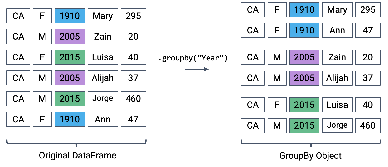
What does this strange output mean? Calling .groupby has generated a GroupBy object. You can imagine this as a set of “mini” sub-DataFrames, where each subframe contains all of the rows from babynames that correspond to a particular year.
The diagram below shows a simplified view of babynames to help illustrate this idea.
Creating a GroupBy object
We can’t work with a GroupBy object directly – that is why you saw that strange output earlier, rather than a standard view of a DataFrame. To actually manipulate values within these “mini” DataFrames, we’ll need to call an aggregation method. This is a method that tells pandas how to aggregate the values within the GroupBy object. Once the aggregation is applied, pandas will return a normal (now grouped) DataFrame.
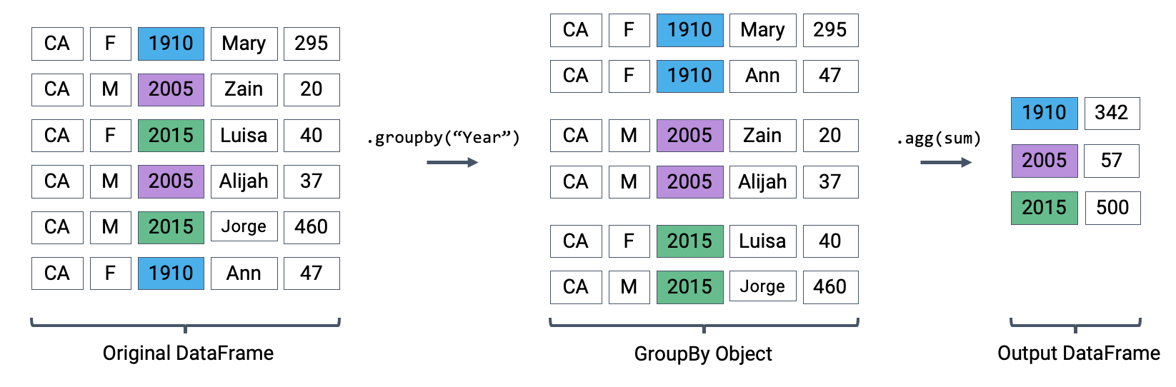
The first aggregation method we’ll consider is .agg. The .agg method takes in a function as its argument; this function is then applied to each column of a “mini” grouped DataFrame. We end up with a new DataFrame with one aggregated row per subframe. Let’s see this in action by finding the sum of all counts for each year in babynames – this is equivalent to finding the number of babies born in each year.
babynames.groupby("Year").agg(sum).head(5)
State
Sex
Name
Count
Year
1910
CACACACACACACACACACACACACACACACACACACACACACACA...
FFFFFFFFFFFFFFFFFFFFFFFFFFFFFFFFFFFFFFFFFFFFFF...
MaryHelenDorothyMargaretFrancesRuthEvelynAlice...
9163
1911
CACACACACACACACACACACACACACACACACACACACACACACA...
FFFFFFFFFFFFFFFFFFFFFFFFFFFFFFFFFFFFFFFFFFFFFF...
MaryDorothyHelenMargaretRuthFrancesAliceEvelyn...
9983
1912
CACACACACACACACACACACACACACACACACACACACACACACA...
FFFFFFFFFFFFFFFFFFFFFFFFFFFFFFFFFFFFFFFFFFFFFF...
MaryDorothyHelenMargaretRuthFrancesAliceVirgin...
17946
1913
CACACACACACACACACACACACACACACACACACACACACACACA...
FFFFFFFFFFFFFFFFFFFFFFFFFFFFFFFFFFFFFFFFFFFFFF...
MaryDorothyHelenMargaretRuthFrancesVirginiaEli...
22094
1914
CACACACACACACACACACACACACACACACACACACACACACACA...
FFFFFFFFFFFFFFFFFFFFFFFFFFFFFFFFFFFFFFFFFFFFFF...
MaryDorothyHelenMargaretRuthFrancesEvelynVirgi...
26926
We can relate this back to the diagram we used above. Remember that the diagram uses a simplified version of babynames, which is why we see smaller values for the summed counts.
Performing an aggregation
Calling .agg has condensed each subframe back into a single row. This gives us our final output: a DataFrame that is now indexed by "Year", with a single row for each unique year in the original babynames DataFrame.
You may be wondering: where did the "State", "Sex", and "Name" columns go? Logically, it doesn’t make sense to sum the string data in these columns (how would we add “Mary” + “Ann”?). Because of this, pandas will simply omit these columns when it performs the aggregation on the DataFrame. Since this happens implicitly, without the user specifying that these columns should be ignored, it’s easy to run into troubling situations where columns are removed without the programmer noticing. It is better coding practice to select only the columns we care about before performing the aggregation.
# Same result, but now we explicitly tell pandas to only consider the "Count" column when summingbabynames.groupby("Year")[["Count"]].agg(sum).head(5)
Count
Year
1910
9163
1911
9983
1912
17946
1913
22094
1914
26926
There are many different aggregations that can be applied to the grouped data. The primary requirement is that an aggregation function must:
Take in a Series of data (a single column of the grouped subframe)
Return a single value that aggregates this Series
Because of this fairly broad requirement, pandas offers many ways of computing an aggregation.
In-built Python operations – such as sum, max, and min – are automatically recognized by pandas.
# What is the maximum count for each name in any year?babynames.groupby("Name")[["Count"]].agg(max).head()
Count
Name
Aadan
7
Aadarsh
6
Aaden
158
Aadhav
8
Aadhira
10
# What is the minimum count for each name in any year?babynames.groupby("Name")[["Count"]].agg(min).head()
Count
Name
Aadan
5
Aadarsh
6
Aaden
10
Aadhav
6
Aadhira
6
As mentioned previously, functions from the NumPy library, such as np.mean, np.max, np.min, and np.sum, are also fair game in pandas.
# What is the average count for each name across all years?babynames.groupby("Name")[["Count"]].agg(np.mean).head()
Count
Name
Aadan
6.000000
Aadarsh
6.000000
Aaden
46.214286
Aadhav
6.750000
Aadhira
7.250000
pandas also offers a number of in-built functions. Functions that are native to pandas can be referenced using their string name within a call to .agg. Some examples include:
.agg("sum")
.agg("max")
.agg("min")
.agg("mean")
.agg("first")
.agg("last")
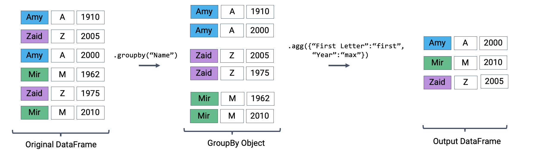
The latter two entries in this list – "first" and "last" – are unique to pandas. They return the first or last entry in a subframe column. Why might this be useful? Consider a case where multiple columns in a group share identical information. To represent this information in the grouped output, we can simply grab the first or last entry, which we know will be identical to all other entries.
Let’s illustrate this with an example. Say we add a new column to babynames that contains the first letter of each name.
# Imagine we had an additional column, "First Letter". We'll explain this code next weekbabynames["First Letter"] = babynames["Name"].str[0]# We construct a simplified DataFrame containing just a subset of columnsbabynames_new = babynames[["Name", "First Letter", "Year"]]babynames_new.head()
Name
First Letter
Year
0
Mary
M
1910
1
Helen
H
1910
2
Dorothy
D
1910
3
Margaret
M
1910
4
Frances
F
1910
If we form groups for each name in the dataset, "First Letter" will be the same for all members of the group. This means that if we simply select the first entry for "First Letter" in the group, we’ll represent all data in that group.
We can use a dictionary to apply different aggregation functions to each column during grouping.
We can also define aggregation functions of our own! This can be done using either a def or lambda statement. Again, the condition for a custom aggregation function is that it must take in a Series and output a single scalar value.
# Alternatively, using lambdababynames.groupby("Name")[["Year", "Count"]].agg(lambda s: s.iloc[-1]/max(s))
Year
Count
Name
Aadan
1.0
0.714286
Aadarsh
1.0
1.000000
Aaden
1.0
0.063291
Aadhav
1.0
0.750000
Aadhira
1.0
0.700000
...
...
...
Zymir
1.0
1.000000
Zyon
1.0
0.933333
Zyra
1.0
1.000000
Zyrah
1.0
0.833333
Zyrus
1.0
1.000000
20239 rows × 2 columns
3.5 Parting Note
Manipulating DataFrames is a skill that is not mastered in just one day. Due to the flexibility of pandas, there are many different ways to get from a point A to a point B. We recommend trying multiple different ways to solve the same problem to gain even more practice and reach that point of mastery sooner.
Next, we will start digging deeper into the mechanics behind grouping data.