3 Pandas II

Important Note

This course note was developed in Fall 2023. If you are taking this class in a future semester, please keep in mind that this note may not be up to date with course content for that semester.

Learning Outcomes

Continue building familiarity with pandas syntax.
Extract data from a DataFrame using conditional selection.
Recognize situations where aggregation is useful and identify the correct technique for performing an aggregation.

Last time, we introduced the pandas library as a toolkit for processing data. We learned the DataFrame and Series data structures, familiarized ourselves with the basic syntax for manipulating tabular data, and began writing our first lines of pandas code.

In this lecture, we’ll start to dive into some advanced pandas syntax. You may find it helpful to follow along with a notebook of your own as we walk through these new pieces of code.

We’ll start by loading the babynames dataset.

Code

# This code pulls census data and loads it into a DataFrame
# We won't cover it explicitly in this class, but you are welcome to explore it on your own
import pandas as pd
import numpy as np
import urllib.request
import os.path
import zipfile

data_url = "https://www.ssa.gov/oact/babynames/state/namesbystate.zip"
local_filename = "data/babynamesbystate.zip"
if not os.path.exists(local_filename): # If the data exists don't download again
    with urllib.request.urlopen(data_url) as resp, open(local_filename, 'wb') as f:
        f.write(resp.read())

zf = zipfile.ZipFile(local_filename, 'r')

ca_name = 'STATE.CA.TXT'
field_names = ['State', 'Sex', 'Year', 'Name', 'Count']
with zf.open(ca_name) as fh:
    babynames = pd.read_csv(fh, header=None, names=field_names)

babynames.head()

	State	Sex	Year	Name	Count
0	CA	F	1910	Mary	295
1	CA	F	1910	Helen	239
2	CA	F	1910	Dorothy	220
3	CA	F	1910	Margaret	163
4	CA	F	1910	Frances	134

3.1 Conditional Selection

Conditional selection allows us to select a subset of rows in a DataFrame that satisfy some specified condition.

To understand how to use conditional selection, we must look at another possible input of the .loc and [] methods – a boolean array, which is simply an array or Series where each element is either True or False. This boolean array must have a length equal to the number of rows in the DataFrame. It will return all rows that correspond to a value of True in the array. We used a very similar technique when performing conditional extraction from a Series in the last lecture.

To see this in action, let’s select all even-indexed rows in the first 10 rows of our DataFrame.

# Ask yourself: why is :9 is the correct slice to select the first 10 rows?
babynames_first_10_rows = babynames.loc[:9, :]

# Notice how we have exactly 10 elements in our boolean array argument
babynames_first_10_rows[[True, False, True, False, True, False, True, False, True, False]]

	State	Sex	Year	Name	Count
0	CA	F	1910	Mary	295
2	CA	F	1910	Dorothy	220
4	CA	F	1910	Frances	134
6	CA	F	1910	Evelyn	126
8	CA	F	1910	Virginia	101

We can perform a similar operation using .loc.

babynames_first_10_rows.loc[[True, False, True, False, True, False, True, False, True, False], :]

	State	Sex	Year	Name	Count
0	CA	F	1910	Mary	295
2	CA	F	1910	Dorothy	220
4	CA	F	1910	Frances	134
6	CA	F	1910	Evelyn	126
8	CA	F	1910	Virginia	101

These techniques worked well in this example, but you can imagine how tedious it might be to list out Trues and Falses for every row in a larger DataFrame. To make things easier, we can instead provide a logical condition as an input to .loc or [] that returns a boolean array with the necessary length.

For example, to return all names associated with F sex:

# First, use a logical condition to generate a boolean array
logical_operator = (babynames["Sex"] == "F")

# Then, use this boolean array to filter the DataFrame
babynames[logical_operator].head()

	State	Sex	Year	Name	Count
0	CA	F	1910	Mary	295
1	CA	F	1910	Helen	239
2	CA	F	1910	Dorothy	220
3	CA	F	1910	Margaret	163
4	CA	F	1910	Frances	134

Recall from the previous lecture that .head() will return only the first few rows in the DataFrame. In reality, babynames[logical operator] contains as many rows as there are entries in the original babynames DataFrame with sex "F".

Here, logical_operator evaluates to a Series of boolean values with length 407428.

Code

print("There are a total of {} values in 'logical_operator'".format(len(logical_operator)))

There are a total of 407428 values in 'logical_operator'

Rows starting at row 0 and ending at row 239536 evaluate to True and are thus returned in the DataFrame. Rows from 239537 onwards evaluate to False and are omitted from the output.

Code

print("The 0th item in this 'logical_operator' is: {}".format(logical_operator.iloc[0]))
print("The 239536th item in this 'logical_operator' is: {}".format(logical_operator.iloc[239536]))
print("The 239537th item in this 'logical_operator' is: {}".format(logical_operator.iloc[239537]))

The 0th item in this 'logical_operator' is: True
The 239536th item in this 'logical_operator' is: True
The 239537th item in this 'logical_operator' is: False

Passing a Series as an argument to babynames[] has the same effect as using a boolean array. In fact, the [] selection operator can take a boolean Series, array, and list as arguments. These three are used interchangeably throughout the course.

We can also use .loc to achieve similar results.

babynames.loc[babynames["Sex"] == "F"].head()

	State	Sex	Year	Name	Count
0	CA	F	1910	Mary	295
1	CA	F	1910	Helen	239
2	CA	F	1910	Dorothy	220
3	CA	F	1910	Margaret	163
4	CA	F	1910	Frances	134

Boolean conditions can be combined using various bitwise operators, allowing us to filter results by multiple conditions. In the table below, p and q are boolean arrays or Series.

Symbol	Usage	Meaning
~	~p	Returns negation of p
\|	p \| q	p OR q
&	p & q	p AND q
^	p ^ q	p XOR q (exclusive or)

When combining multiple conditions with logical operators, we surround each individual condition with a set of parenthesis (). This imposes an order of operations on pandas evaluating your logic and can avoid code erroring.

For example, if we want to return data on all names with sex "F" born before the year 2000, we can write:

babynames[(babynames["Sex"] == "F") & (babynames["Year"] < 2000)].head()

	State	Sex	Year	Name	Count
0	CA	F	1910	Mary	295
1	CA	F	1910	Helen	239
2	CA	F	1910	Dorothy	220
3	CA	F	1910	Margaret	163
4	CA	F	1910	Frances	134

If we want to return data on all names with sex "F" or all born before the year 2000, we can write:

babynames[(babynames["Sex"] == "F") | (babynames["Year"] < 2000)].head()

	State	Sex	Year	Name	Count
0	CA	F	1910	Mary	295
1	CA	F	1910	Helen	239
2	CA	F	1910	Dorothy	220
3	CA	F	1910	Margaret	163
4	CA	F	1910	Frances	134

Boolean array selection is a useful tool, but can lead to overly verbose code for complex conditions. In the example below, our boolean condition is long enough to extend for several lines of code.

# Note: The parentheses surrounding the code make it possible to break the code on to multiple lines for readability
(
    babynames[(babynames["Name"] == "Bella") | 
              (babynames["Name"] == "Alex") |
              (babynames["Name"] == "Ani") |
              (babynames["Name"] == "Lisa")]
).head()

	State	Sex	Year	Name	Count
6289	CA	F	1923	Bella	5
7512	CA	F	1925	Bella	8
12368	CA	F	1932	Lisa	5
14741	CA	F	1936	Lisa	8
17084	CA	F	1939	Lisa	5

Fortunately, pandas provides many alternative methods for constructing boolean filters.

The .isin function is one such example. This method evaluates if the values in a Series are contained in a different sequence (list, array, or Series) of values. In the cell below, we achieve equivalent results to the DataFrame above with far more concise code.

names = ["Bella", "Alex", "Narges", "Lisa"]
babynames["Name"].isin(names).head()

0    False
1    False
2    False
3    False
4    False
Name: Name, dtype: bool

babynames[babynames["Name"].isin(names)].head()

	State	Sex	Year	Name	Count
6289	CA	F	1923	Bella	5
7512	CA	F	1925	Bella	8
12368	CA	F	1932	Lisa	5
14741	CA	F	1936	Lisa	8
17084	CA	F	1939	Lisa	5

The function str.startswith can be used to define a filter based on string values in a Series object. It checks to see if string values in a Series start with a particular character.

# Identify whether names begin with the letter "N"
babynames["Name"].str.startswith("N").head()

0    False
1    False
2    False
3    False
4    False
Name: Name, dtype: bool

# Extracting names that begin with the letter "N"
babynames[babynames["Name"].str.startswith("N")].head()

	State	Sex	Year	Name	Count
76	CA	F	1910	Norma	23
83	CA	F	1910	Nellie	20
127	CA	F	1910	Nina	11
198	CA	F	1910	Nora	6
310	CA	F	1911	Nellie	23

3.2 Adding, Removing, and Modifying Columns

In many data science tasks, we may need to change the columns contained in our DataFrame in some way. Fortunately, the syntax to do so is fairly straightforward.

To add a new column to a DataFrame, we use a syntax similar to that used when accessing an existing column. Specify the name of the new column by writing df["column"], then assign this to a Series or array containing the values that will populate this column.

# Create a Series of the length of each name. 
babyname_lengths = babynames["Name"].str.len()

# Add a column named "name_lengths" that includes the length of each name
babynames["name_lengths"] = babyname_lengths
babynames.head(5)

	State	Sex	Year	Name	Count	name_lengths
0	CA	F	1910	Mary	295	4
1	CA	F	1910	Helen	239	5
2	CA	F	1910	Dorothy	220	7
3	CA	F	1910	Margaret	163	8
4	CA	F	1910	Frances	134	7

If we need to later modify an existing column, we can do so by referencing this column again with the syntax df["column"], then re-assigning it to a new Series or array of the appropriate length.

# Modify the “name_lengths” column to be one less than its original value
babynames["name_lengths"] = babynames["name_lengths"] - 1
babynames.head()

	State	Sex	Year	Name	Count	name_lengths
0	CA	F	1910	Mary	295	3
1	CA	F	1910	Helen	239	4
2	CA	F	1910	Dorothy	220	6
3	CA	F	1910	Margaret	163	7
4	CA	F	1910	Frances	134	6

We can rename a column using the .rename() method. .rename() takes in a dictionary that maps old column names to their new ones.

# Rename “name_lengths” to “Length”
babynames = babynames.rename(columns={"name_lengths":"Length"})
babynames.head()

	State	Sex	Year	Name	Count	Length
0	CA	F	1910	Mary	295	3
1	CA	F	1910	Helen	239	4
2	CA	F	1910	Dorothy	220	6
3	CA	F	1910	Margaret	163	7
4	CA	F	1910	Frances	134	6

If we want to remove a column or row of a DataFrame, we can call the .drop method. Use the axis parameter to specify whether a column or row should be dropped. Unless otherwise specified, pandas will assume that we are dropping a row by default.

# Drop our new "Length" column from the DataFrame
babynames = babynames.drop("Length", axis="columns")
babynames.head(5)

	State	Sex	Year	Name	Count
0	CA	F	1910	Mary	295
1	CA	F	1910	Helen	239
2	CA	F	1910	Dorothy	220
3	CA	F	1910	Margaret	163
4	CA	F	1910	Frances	134

Notice that we re-assigned babynames to the result of babynames.drop(...). This is a subtle but important point: pandas table operations do not occur in-place. Calling df.drop(...) will output a copy of df with the row/column of interest removed without modifying the original df table.

In other words, if we simply call:

# This creates a copy of `babynames` and removes the column "Name"...
babynames.drop("Name", axis="columns")

# ...but the original `babynames` is unchanged! 
# Notice that the "Name" column is still present
babynames.head(5)

	State	Sex	Year	Name	Count
0	CA	F	1910	Mary	295
1	CA	F	1910	Helen	239
2	CA	F	1910	Dorothy	220
3	CA	F	1910	Margaret	163
4	CA	F	1910	Frances	134

3.3 Handy Utility Functions

pandas contains an extensive library of functions that can help shorten the process of setting and getting information from its data structures. In the following section, we will give overviews of each of the main utility functions that will help us in Data 100.

Discussing all functionality offered by pandas could take an entire semester! We will walk you through the most commonly-used functions and encourage you to explore and experiment on your own.

NumPy and built-in function support
.shape
.size
.describe()
.sample()
.value_counts()
.unique()
.sort_values()

The pandas documentation will be a valuable resource in Data 100 and beyond.

3.3.1 `NumPy`

pandas is designed to work well with NumPy, the framework for array computations you encountered in Data 8. Just about any NumPy function can be applied to pandas DataFrames and Series.

# Pull out the number of babies named Yash each year
yash_count = babynames[babynames["Name"] == "Yash"]["Count"]
yash_count.head()

331824     8
334114     9
336390    11
338773    12
341387    10
Name: Count, dtype: int64

# Average number of babies named Yash each year
np.mean(yash_count)

17.142857142857142

# Max number of babies named Yash born in any one year
np.max(yash_count)

3.3.2 `.shape` and `.size`

.shape and .size are attributes of Series and DataFrames that measure the “amount” of data stored in the structure. Calling .shape returns a tuple containing the number of rows and columns present in the DataFrame or Series. .size is used to find the total number of elements in a structure, equivalent to the number of rows times the number of columns.

Many functions strictly require the dimensions of the arguments along certain axes to match. Calling these dimension-finding functions is much faster than counting all of the items by hand.

# Return the shape of the DataFrame, in the format (num_rows, num_columns)
babynames.shape

(407428, 5)

# Return the size of the DataFrame, equal to num_rows * num_columns
babynames.size

3.3.3 `.describe()`

If many statistics are required from a DataFrame (minimum value, maximum value, mean value, etc.), then .describe() can be used to compute all of them at once.

babynames.describe()

	Year	Count
count	407428.000000	407428.000000
mean	1985.733609	79.543456
std	27.007660	293.698654
min	1910.000000	5.000000
25%	1969.000000	7.000000
50%	1992.000000	13.000000
75%	2008.000000	38.000000
max	2022.000000	8260.000000

A different set of statistics will be reported if .describe() is called on a Series.

babynames["Sex"].describe()

count     407428
unique         2
top            F
freq      239537
Name: Sex, dtype: object

3.3.4 `.sample()`

As we will see later in the semester, random processes are at the heart of many data science techniques (for example, train-test splits, bootstrapping, and cross-validation). .sample() lets us quickly select random entries (a row if called from a DataFrame, or a value if called from a Series).

By default, .sample() selects entries without replacement. Pass in the argument replace=True to sample with replacement.

# Sample a single row
babynames.sample()

	State	Sex	Year	Name	Count
126330	CA	F	1993	Ronisha	8

Naturally, this can be chained with other methods and operators (iloc, etc.).

# Sample 5 random rows, and select all columns after column 2
babynames.sample(5).iloc[:, 2:]

	Year	Name	Count
287195	1972	Maceo	5
263477	1952	Sean	38
384300	2014	Sahas	5
71392	1974	Shae	5
88968	1982	Delia	63

# Randomly sample 4 names from the year 2000, with replacement, and select all columns after column 2
babynames[babynames["Year"] == 2000].sample(4, replace = True).iloc[:, 2:]

	Year	Name	Count
343579	2000	Anson	13
344950	2000	Yoni	5
344594	2000	Yahya	6
150348	2000	Betty	20

3.3.5 `.value_counts()`

The Series.value_counts() method counts the number of occurrence of each unique value in a Series. In other words, it counts the number of times each unique value appears. This is often useful for determining the most or least common entries in a Series.

In the example below, we can determine the name with the most years in which at least one person has taken that name by counting the number of times each name appears in the "Name" column of babynames. Note that the return value is also a Series.

babynames["Name"].value_counts().head()

Jean         223
Francis      221
Guadalupe    218
Jessie       217
Marion       214
Name: Name, dtype: int64

3.3.6 `.unique()`

If we have a Series with many repeated values, then .unique() can be used to identify only the unique values. Here we return an array of all the names in babynames.

babynames["Name"].unique()

array(['Mary', 'Helen', 'Dorothy', ..., 'Zae', 'Zai', 'Zayvier'],
      dtype=object)

3.3.7 `.sort_values()`

Ordering a DataFrame can be useful for isolating extreme values. For example, the first 5 entries of a row sorted in descending order (that is, from highest to lowest) are the largest 5 values. .sort_values allows us to order a DataFrame or Series by a specified column. We can choose to either receive the rows in ascending order (default) or descending order.

# Sort the "Count" column from highest to lowest
babynames.sort_values(by="Count", ascending=False).head()

	State	Sex	Year	Name	Count
268041	CA	M	1957	Michael	8260
267017	CA	M	1956	Michael	8258
317387	CA	M	1990	Michael	8246
281850	CA	M	1969	Michael	8245
283146	CA	M	1970	Michael	8196

Unlike when calling .value_counts() on a DataFrame, we do not need to explicitly specify the column used for sorting when calling .value_counts() on a Series. We can still specify the ordering paradigm – that is, whether values are sorted in ascending or descending order.

# Sort the "Name" Series alphabetically
babynames["Name"].sort_values(ascending=True).head()

366001      Aadan
384005      Aadan
369120      Aadan
398211    Aadarsh
370306      Aaden
Name: Name, dtype: object

3.4 Custom Sorts

Let’s now try applying what we’ve just learned to solve a sorting problem using different approaches. Assume we want to find the longest baby names and sort our data accordingly.

3.4.1 Approach 1: Create a Temporary Column

One method to do this is to first start by creating a column that contains the lengths of the names.

# Create a Series of the length of each name
babyname_lengths = babynames["Name"].str.len()

# Add a column named "name_lengths" that includes the length of each name
babynames["name_lengths"] = babyname_lengths
babynames.head(5)

	State	Sex	Year	Name	Count	name_lengths
0	CA	F	1910	Mary	295	4
1	CA	F	1910	Helen	239	5
2	CA	F	1910	Dorothy	220	7
3	CA	F	1910	Margaret	163	8
4	CA	F	1910	Frances	134	7

We can then sort the DataFrame by that column using .sort_values():

# Sort by the temporary column
babynames = babynames.sort_values(by="name_lengths", ascending=False)
babynames.head(5)

	State	Sex	Year	Name	Count	name_lengths
334166	CA	M	1996	Franciscojavier	8	15
337301	CA	M	1997	Franciscojavier	5	15
339472	CA	M	1998	Franciscojavier	6	15
321792	CA	M	1991	Ryanchristopher	7	15
327358	CA	M	1993	Johnchristopher	5	15

Finally, we can drop the name_length column from babynames to prevent our table from getting cluttered.

# Drop the 'name_length' column
babynames = babynames.drop("name_lengths", axis='columns')
babynames.head(5)

	State	Sex	Year	Name	Count
334166	CA	M	1996	Franciscojavier	8
337301	CA	M	1997	Franciscojavier	5
339472	CA	M	1998	Franciscojavier	6
321792	CA	M	1991	Ryanchristopher	7
327358	CA	M	1993	Johnchristopher	5

3.4.2 Approach 2: Sorting using the `key` Argument

Another way to approach this is to use the key argument of .sort_values(). Here we can specify that we want to sort "Name" values by their length.

babynames.sort_values("Name", key=lambda x: x.str.len(), ascending=False).head()

	State	Sex	Year	Name	Count
334166	CA	M	1996	Franciscojavier	8
327472	CA	M	1993	Ryanchristopher	5
337301	CA	M	1997	Franciscojavier	5
337477	CA	M	1997	Ryanchristopher	5
312543	CA	M	1987	Franciscojavier	5

3.4.3 Approach 3: Sorting using the `map` Function

We can also use the map function on a Series to solve this. Say we want to sort the babynames table by the number of "dr"’s and "ea"s in each "Name". We’ll define the function dr_ea_count to help us out.

# First, define a function to count the number of times "dr" or "ea" appear in each name
def dr_ea_count(string):
    return string.count('dr') + string.count('ea')

# Then, use `map` to apply `dr_ea_count` to each name in the "Name" column
babynames["dr_ea_count"] = babynames["Name"].map(dr_ea_count)

# Sort the DataFrame by the new "dr_ea_count" column so we can see our handiwork
babynames = babynames.sort_values(by="dr_ea_count", ascending=False)
babynames.head()

	State	Sex	Year	Name	Count	dr_ea_count
115957	CA	F	1990	Deandrea	5	3
101976	CA	F	1986	Deandrea	6	3
131029	CA	F	1994	Leandrea	5	3
108731	CA	F	1988	Deandrea	5	3
308131	CA	M	1985	Deandrea	6	3

We can drop the dr_ea_count once we’re done using it to maintain a neat table.

# Drop the `dr_ea_count` column
babynames = babynames.drop("dr_ea_count", axis = 'columns')
babynames.head(5)

	State	Sex	Year	Name	Count
115957	CA	F	1990	Deandrea	5
101976	CA	F	1986	Deandrea	6
131029	CA	F	1994	Leandrea	5
108731	CA	F	1988	Deandrea	5
308131	CA	M	1985	Deandrea	6

3.5 Aggregating Data with `.groupby`

Up until this point, we have been working with individual rows of DataFrames. As data scientists, we often wish to investigate trends across a larger subset of our data. For example, we may want to compute some summary statistic (the mean, median, sum, etc.) for a group of rows in our DataFrame. To do this, we’ll use pandas GroupBy objects.

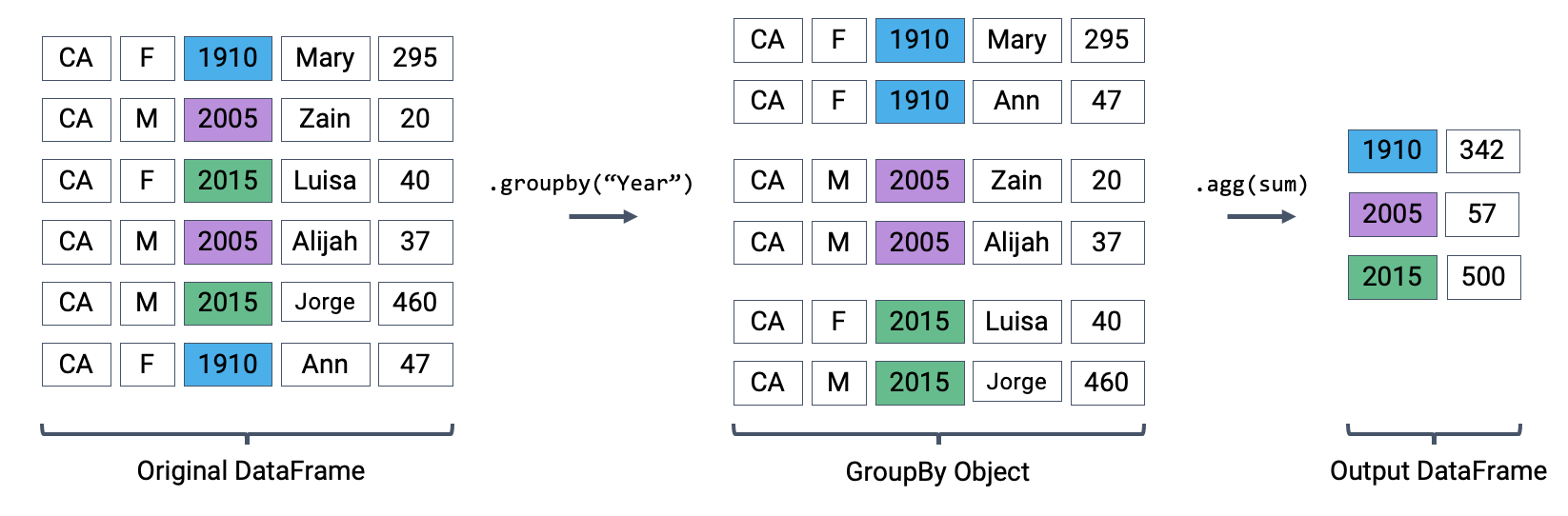
Let’s say we wanted to aggregate all rows in babynames for a given year.

babynames.groupby("Year")

<pandas.core.groupby.generic.DataFrameGroupBy object at 0x1258f1250>

What does this strange output mean? Calling .groupby has generated a GroupBy object. You can imagine this as a set of “mini” sub-DataFrames, where each subframe contains all of the rows from babynames that correspond to a particular year.

The diagram below shows a simplified view of babynames to help illustrate this idea.

We can’t work with a GroupBy object directly – that is why you saw that strange output earlier rather than a standard view of a DataFrame. To actually manipulate values within these “mini” DataFrames, we’ll need to call an aggregation method. This is a method that tells pandas how to aggregate the values within the GroupBy object. Once the aggregation is applied, pandas will return a normal (now grouped) DataFrame.

The first aggregation method we’ll consider is .agg. The .agg method takes in a function as its argument; this function is then applied to each column of a “mini” grouped DataFrame. We end up with a new DataFrame with one aggregated row per subframe. Let’s see this in action by finding the sum of all counts for each year in babynames – this is equivalent to finding the number of babies born in each year.

babynames[["Year", "Count"]].groupby("Year").agg(sum).head(5)

	Count
Year
1910	9163
1911	9983
1912	17946
1913	22094
1914	26926

We can relate this back to the diagram we used above. Remember that the diagram uses a simplified version of babynames, which is why we see smaller values for the summed counts.

Calling .agg has condensed each subframe back into a single row. This gives us our final output: a DataFrame that is now indexed by "Year", with a single row for each unique year in the original babynames DataFrame.

You may be wondering: where did the "State", "Sex", and "Name" columns go? Logically, it doesn’t make sense to sum the string data in these columns (how would we add “Mary” + “Ann”?). Because of this, we need to omit these columns when we perform aggregation on the DataFrame.

# Same result, but now we explicitly tell pandas to only consider the "Count" column when summing
babynames.groupby("Year")[["Count"]].agg(sum).head(5)

	Count
Year
1910	9163
1911	9983
1912	17946
1913	22094
1914	26926

There are many different aggregations that can be applied to the grouped data. The primary requirement is that an aggregation function must:

Take in a Series of data (a single column of the grouped subframe).
Return a single value that aggregates this Series.

Because of this fairly broad requirement, pandas offers many ways of computing an aggregation.

In-built Python operations – such as sum, max, and min – are automatically recognized by pandas.

# What is the minimum count for each name in any year?
babynames.groupby("Name")[["Count"]].agg(min).head()

	Count
Name
Aadan	5
Aadarsh	6
Aaden	10
Aadhav	6
Aadhini	6

# What is the largest single-year count of each name?
babynames.groupby("Name")[["Count"]].agg(max).head()

	Count
Name
Aadan	7
Aadarsh	6
Aaden	158
Aadhav	8
Aadhini	6

As mentioned previously, functions from the NumPy library, such as np.mean, np.max, np.min, and np.sum, are also fair game in pandas.

# What is the average count for each name across all years?
babynames.groupby("Name")[["Count"]].agg(np.mean).head()

	Count
Name
Aadan	6.000000
Aadarsh	6.000000
Aaden	46.214286
Aadhav	6.750000
Aadhini	6.000000

pandas also offers a number of in-built functions. Functions that are native to pandas can be referenced using their string name within a call to .agg. Some examples include:

.agg("sum")
.agg("max")
.agg("min")
.agg("mean")
.agg("first")
.agg("last")

The latter two entries in this list – "first" and "last" – are unique to pandas. They return the first or last entry in a subframe column. Why might this be useful? Consider a case where multiple columns in a group share identical information. To represent this information in the grouped output, we can simply grab the first or last entry, which we know will be identical to all other entries.

Let’s illustrate this with an example. Say we add a new column to babynames that contains the first letter of each name.

# Imagine we had an additional column, "First Letter". We'll explain this code next week
babynames["First Letter"] = babynames["Name"].str[0]

# We construct a simplified DataFrame containing just a subset of columns
babynames_new = babynames[["Name", "First Letter", "Year"]]
babynames_new.head()

	Name	First Letter	Year
115957	Deandrea	D	1990
101976	Deandrea	D	1986
131029	Leandrea	L	1994
108731	Deandrea	D	1988
308131	Deandrea	D	1985

If we form groups for each name in the dataset, "First Letter" will be the same for all members of the group. This means that if we simply select the first entry for "First Letter" in the group, we’ll represent all data in that group.

We can use a dictionary to apply different aggregation functions to each column during grouping.

babynames_new.groupby("Name").agg({"First Letter":"first", "Year":"max"}).head()

	First Letter	Year
Name
Aadan	A	2014
Aadarsh	A	2019
Aaden	A	2020
Aadhav	A	2019
Aadhini	A	2022

Some aggregation functions are common enough that pandas allows them to be called directly, without the explicit use of .agg.

babynames.groupby("Name")[["Count"]].mean().head()

	Count
Name
Aadan	6.000000
Aadarsh	6.000000
Aaden	46.214286
Aadhav	6.750000
Aadhini	6.000000

We can also define aggregation functions of our own! This can be done using either a def or lambda statement. Again, the condition for a custom aggregation function is that it must take in a Series and output a single scalar value.

babynames = babynames.sort_values(by="Year", ascending=True)
def ratio_to_peak(series):
    return series.iloc[-1]/max(series)

babynames.groupby("Name")[["Year", "Count"]].agg(ratio_to_peak)

	Year	Count
Name
Aadan	1.0	0.714286
Aadarsh	1.0	1.000000
Aaden	1.0	0.063291
Aadhav	1.0	0.750000
Aadhini	1.0	1.000000
...	...	...
Zymir	1.0	1.000000
Zyon	1.0	1.000000
Zyra	1.0	1.000000
Zyrah	1.0	0.833333
Zyrus	1.0	1.000000

20437 rows × 2 columns

# Alternatively, using lambda
babynames.groupby("Name")[["Year", "Count"]].agg(lambda s: s.iloc[-1]/max(s))

	Year	Count
Name
Aadan	1.0	0.714286
Aadarsh	1.0	1.000000
Aaden	1.0	0.063291
Aadhav	1.0	0.750000
Aadhini	1.0	1.000000
...	...	...
Zymir	1.0	1.000000
Zyon	1.0	1.000000
Zyra	1.0	1.000000
Zyrah	1.0	0.833333
Zyrus	1.0	1.000000

20437 rows × 2 columns

3.6 Parting Note

Manipulating DataFrames is not a skill that is mastered in just one day. Due to the flexibility of pandas, there are many different ways to get from point A to point B. We recommend trying multiple different ways to solve the same problem to gain even more practice and reach that point of mastery sooner.

Next, we will start digging deeper into the mechanics behind grouping data.

3.1 Conditional Selection

3.2 Adding, Removing, and Modifying Columns

3.3 Handy Utility Functions

3.3.1 NumPy

3.3.2 .shape and .size

3.3.3 .describe()

3.3.4 .sample()

3.3.5 .value_counts()

3.3.6 .unique()

3.3.7 .sort_values()

3.4 Custom Sorts

3.4.1 Approach 1: Create a Temporary Column

3.4.2 Approach 2: Sorting using the key Argument

3.4.3 Approach 3: Sorting using the map Function

3.5 Aggregating Data with .groupby

3.6 Parting Note

3.3.1 `NumPy`

3.3.2 `.shape` and `.size`

3.3.3 `.describe()`

3.3.4 `.sample()`

3.3.5 `.value_counts()`

3.3.6 `.unique()`

3.3.7 `.sort_values()`

3.4.2 Approach 2: Sorting using the `key` Argument

3.4.3 Approach 3: Sorting using the `map` Function

3.5 Aggregating Data with `.groupby`