import pandas as pd
import seaborn as sns
import matplotlib.pyplot as plt
import numpy as np
import yaml
from datetime import datetime
from ds100_utils import *
import plotly.express as px
# Reduce number of sigfigs shown by numpy
np.set_printoptions(precision=2, suppress=True)
# Reduce number of sigfigs shown by pandas
pd.set_option('display.float_format', lambda x: '%.2f' % x)
PCA with SVD
Looking at this rectangle data, we can see that it is rank 3, since perimeter
is a linear combination of width and height.
Area is not a linear combination of width and height, but we might surmise that area does not provide a lot of additional information beyond width and height. Let's see if PCA picks up on this.
rectangle = pd.read_csv("data/rectangle_data.csv")
rectangle
| width | height | area | perimeter | |
|---|---|---|---|---|
| 0 | 8 | 6 | 48 | 28 |
| 1 | 2 | 4 | 8 | 12 |
| 2 | 1 | 3 | 3 | 8 |
| 3 | 9 | 3 | 27 | 24 |
| 4 | 9 | 8 | 72 | 34 |
| ... | ... | ... | ... | ... |
| 95 | 8 | 5 | 40 | 26 |
| 96 | 8 | 7 | 56 | 30 |
| 97 | 1 | 4 | 4 | 10 |
| 98 | 1 | 6 | 6 | 14 |
| 99 | 2 | 6 | 12 | 16 |
100 rows × 4 columns
Step 1: Center the Data Matrix $X$
Keep in mind that sklearn centers data by default when fitting PCA. Here,
we are doing the linear algebra by hand.
X_centered = rectangle - np.mean(rectangle, axis = 0)
X_centered.head(10)
| width | height | area | perimeter | |
|---|---|---|---|---|
| 0 | 2.97 | 1.35 | 24.78 | 8.64 |
| 1 | -3.03 | -0.65 | -15.22 | -7.36 |
| 2 | -4.03 | -1.65 | -20.22 | -11.36 |
| 3 | 3.97 | -1.65 | 3.78 | 4.64 |
| 4 | 3.97 | 3.35 | 48.78 | 14.64 |
| 5 | -2.03 | -3.65 | -20.22 | -11.36 |
| 6 | -1.03 | -2.65 | -15.22 | -7.36 |
| 7 | 0.97 | 0.35 | 6.78 | 2.64 |
| 8 | 1.97 | -3.65 | -16.22 | -3.36 |
| 9 | 2.97 | -2.65 | -7.22 | 0.64 |
In situations where the units are on different scales, it is useful to normalize (i.e., standardize) the data before performing SVD. This can be done by dividing each column by its standard deviation.
- This puts every column on a standard deviation scale. A value of 1 implies the entry is 1 standard deviation higher than its mean.
X = X_centered / np.std(X_centered, axis = 0)
X.head(10)
| width | height | area | perimeter | |
|---|---|---|---|---|
| 0 | 1.07 | 0.58 | 1.35 | 1.21 |
| 1 | -1.09 | -0.28 | -0.83 | -1.03 |
| 2 | -1.45 | -0.71 | -1.10 | -1.59 |
| 3 | 1.43 | -0.71 | 0.21 | 0.65 |
| 4 | 1.43 | 1.45 | 2.65 | 2.05 |
| 5 | -0.73 | -1.58 | -1.10 | -1.59 |
| 6 | -0.37 | -1.15 | -0.83 | -1.03 |
| 7 | 0.35 | 0.15 | 0.37 | 0.37 |
| 8 | 0.71 | -1.58 | -0.88 | -0.47 |
| 9 | 1.07 | -1.15 | -0.39 | 0.09 |
Step 2: Get the SVD of standardized $X$
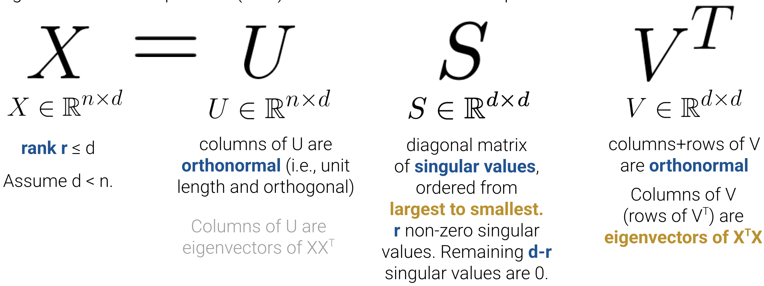
The np.linalg.svd function computes the SVD of an inputted X matrix.
U, S, Vt = np.linalg.svd(X, full_matrices = False)
full_matrices = Falsetruncates the number of columns of U to the rank of X to avoid unnecessary computation. PCA does not use more columns of U than the rank of X. This is sometimes called the "economy" SVD. The slides use the dimensions of the economy SVD. Don't worry about these details for Data 100! Just include the argument.
SVD dimensions:
print("Shape of U", U.shape)
print("Shape of S", S.shape)
print("Shape of Vt", Vt.shape)
Shape of U (100, 4) Shape of S (4,) Shape of Vt (4, 4)
print('First 10 rows of U. The 4 cols are the latent features but expressed as length 1 vectors.')
print(U[:10, :])
print()
print('S. The 4 singular values that "scale up" the 4 cols of U into the 4 latent features (Z).')
print(S)
print()
print('Vt. The 4 rows are the principal components. "Recipes" for combining the 4 real features into each of the 4 latent features. Rows and columns are unit vectors.')
print(Vt)
print()
First 10 rows of U. The 4 cols are the latent features but expressed as length 1 vectors. [[-0.13 0.02 0.05 0.61] [ 0.1 -0.05 0.04 0.04] [ 0.14 -0.04 0.12 -0.06] [-0.05 0.15 -0.1 -0.08] [-0.23 -0.02 0.18 -0.11] [ 0.15 0.07 0.14 -0.05] [ 0.1 0.06 0.06 -0.04] [-0.04 0.01 0. -0.07] [ 0.06 0.16 -0.1 -0.1 ] [ 0.01 0.16 -0.11 -0.07]] S. The 4 singular values that "scale up" the 4 cols of U into the 4 latent features (Z). [16.99 10.13 2.94 0. ] Vt. The 4 rows are the principal components. "Recipes" for combining the 4 real features into each of the 4 latent features. Rows and columns are unit vectors. [[-0.44 -0.38 -0.57 -0.58] [ 0.65 -0.76 -0.02 0.02] [-0.28 -0.28 0.82 -0.41] [ 0.55 0.46 -0. -0.7 ]]
$S$ is a little different in NumPy. Since the only useful values in the diagonal matrix $S$ are the singular values on the diagonal axis, only those values are returned and they are stored in an array.
If we want the diagonal elements:
# np.diag makes a diagonal matrix from the vector S
Sm = np.diag(S)
Sm
array([[16.99, 0. , 0. , 0. ],
[ 0. , 10.13, 0. , 0. ],
[ 0. , 0. , 2.94, 0. ],
[ 0. , 0. , 0. , 0. ]])
Computing the contribution to the total variance:
pd.DataFrame(S**2 / np.sum(S**2))
| 0 | |
|---|---|
| 0 | 0.72 |
| 1 | 0.26 |
| 2 | 0.02 |
| 3 | 0.00 |
Now we see that 72% and 26% of the variance is in the first two PC dimensions, respectively, which makes sense since rectangles are largely described by height and length.
Area is not a linear combination of height and length, so its contribution is non-zero but very small.
Perimeter is a linear combination of height and length, so its corresponding singular value is 0.
The information below is only relevant if you print out all digits with numpy. We set an option at the top of the notebook to only shown two decimal places.
Hmm, looks like are four diagonal entries are not zero. What happened?
It turns out there were some numerical rounding errors, but the last value is so small ($10^{-15}$) that it's practically $0$.
np.isclose(S[3], 0)
np.True_
S.round(5)
array([16.99, 10.13, 2.94, 0. ])
pd.DataFrame(np.round(np.diag(S),3))
| 0 | 1 | 2 | 3 | |
|---|---|---|---|---|
| 0 | 16.99 | 0.00 | 0.00 | 0.00 |
| 1 | 0.00 | 10.13 | 0.00 | 0.00 |
| 2 | 0.00 | 0.00 | 2.94 | 0.00 |
| 3 | 0.00 | 0.00 | 0.00 | 0.00 |
Step 3 Computing Approximations to the Data
Let's try to approximate the data X in two dimensions.
Using $Z = X * V$
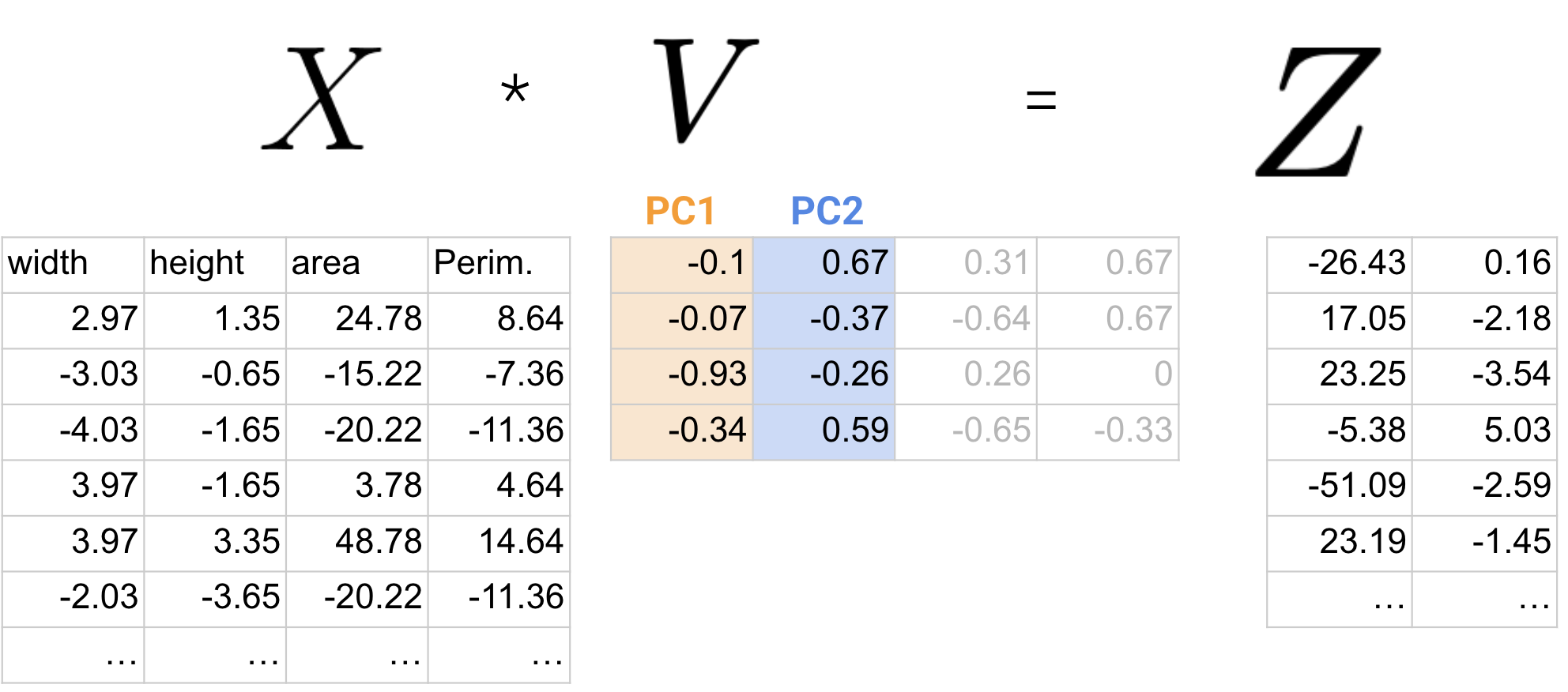
Recall that the columns of Z are the latent features.
The first column of Z is the latent feature with the largest variance, and the second column of Z is the latent feature with the second largest variance that is orthogonal to the first column.
In this example, Z has the same dimensions as the first two columns of X.
# We can construct Z using the V matrix (transpose Vt!)
# The columns of V are the PCs, so the rows of Vt are the PCs.
print('X (truncated):')
print(X.head())
print()
print('Vt:')
print(Vt)
print()
X (truncated): width height area perimeter 0 1.07 0.58 1.35 1.21 1 -1.09 -0.28 -0.83 -1.03 2 -1.45 -0.71 -1.10 -1.59 3 1.43 -0.71 0.21 0.65 4 1.43 1.45 2.65 2.05 Vt: [[-0.44 -0.38 -0.57 -0.58] [ 0.65 -0.76 -0.02 0.02] [-0.28 -0.28 0.82 -0.41] [ 0.55 0.46 -0. -0.7 ]]
# Construct Z using only the first two PCs
Z = X.to_numpy() @ Vt.T[:,:2]
pd.DataFrame(Z).head(10)
| 0 | 1 | |
|---|---|---|
| 0 | -2.17 | 0.25 |
| 1 | 1.66 | -0.50 |
| 2 | 2.46 | -0.42 |
| 3 | -0.86 | 1.48 |
| 4 | -3.88 | -0.18 |
| 5 | 2.47 | 0.71 |
| 6 | 1.67 | 0.62 |
| 7 | -0.64 | 0.11 |
| 8 | 1.06 | 1.67 |
| 9 | 0.13 | 1.58 |
print('First two columns of U (truncated):')
print(U[:10, :2])
print()
print('S:')
np.diag(S[:2])
First two columns of U (truncated): [[-0.13 0.02] [ 0.1 -0.05] [ 0.14 -0.04] [-0.05 0.15] [-0.23 -0.02] [ 0.15 0.07] [ 0.1 0.06] [-0.04 0.01] [ 0.06 0.16] [ 0.01 0.16]] S:
array([[16.99, 0. ],
[ 0. , 10.13]])
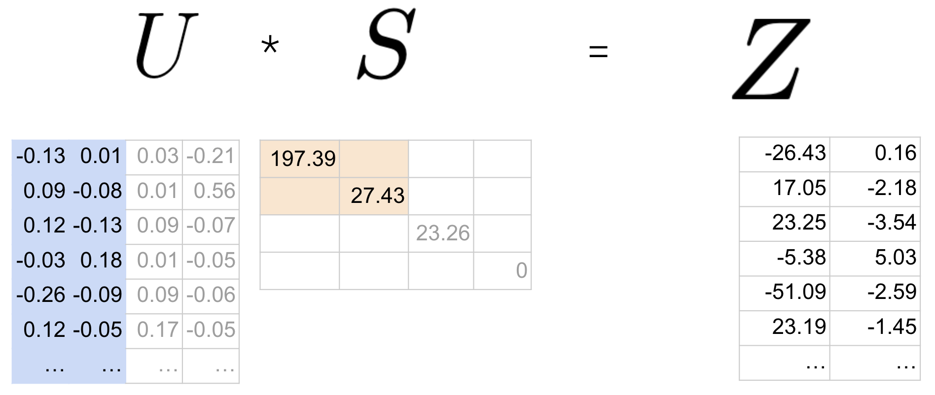
Construct Z using the first two columns of U and the first two singular values:
Z = U[:, :2] @ np.diag(S[:2])
print(Z.shape)
pd.DataFrame(Z).head(10)
(100, 2)
| 0 | 1 | |
|---|---|---|
| 0 | -2.17 | 0.25 |
| 1 | 1.66 | -0.50 |
| 2 | 2.46 | -0.42 |
| 3 | -0.86 | 1.48 |
| 4 | -3.88 | -0.18 |
| 5 | 2.47 | 0.71 |
| 6 | 1.67 | 0.62 |
| 7 | -0.64 | 0.11 |
| 8 | 1.06 | 1.67 |
| 9 | 0.13 | 1.58 |
The columns of U are just the normalized (i.e., length 1) columns of Z:
# Normalize first column of Z using L2 norm
length_of_col_1 = np.sqrt(np.sum(Z[:, 0]**2))
normed_z = Z[:, 0] / length_of_col_1
print(normed_z[:10])
print(U[:10, 0])
[-0.13 0.1 0.14 -0.05 -0.23 0.15 0.1 -0.04 0.06 0.01] [-0.13 0.1 0.14 -0.05 -0.23 0.15 0.1 -0.04 0.06 0.01]
This implies that the singular values are just the length of the column vectors of Z:
# length of first column of Z (L2 norm)
print(np.sqrt(np.sum(Z[:, 0]**2)))
# Identical to code above
print(np.linalg.norm(Z[:, 0]))
# Print first singular value
print(S[0])
16.989286229589222 16.989286229589222 16.98928622958922
We get the same results if we fit PCA with scikit-learn:
from sklearn.decomposition import PCA
# This code computes first two columns of Z (i.e., the first two latent features)
# And, yes, this whole lecture can be summarized by these two lines of code!
# Initialize a PCA model object with 2 components
pca = PCA(2)
# Fit the PCA model to the data
pd.DataFrame(pca.fit_transform(X)).head(10)
| 0 | 1 | |
|---|---|---|
| 0 | 2.17 | -0.25 |
| 1 | -1.66 | 0.50 |
| 2 | -2.46 | 0.42 |
| 3 | 0.86 | -1.48 |
| 4 | 3.88 | 0.18 |
| 5 | -2.47 | -0.71 |
| 6 | -1.67 | -0.62 |
| 7 | 0.64 | -0.11 |
| 8 | -1.06 | -1.67 |
| 9 | -0.13 | -1.58 |
The Z we computed is identical to the one from sklearn:
pd.DataFrame(Z).head(10)
| 0 | 1 | |
|---|---|---|
| 0 | -2.17 | 0.25 |
| 1 | 1.66 | -0.50 |
| 2 | 2.46 | -0.42 |
| 3 | -0.86 | 1.48 |
| 4 | -3.88 | -0.18 |
| 5 | 2.47 | 0.71 |
| 6 | 1.67 | 0.62 |
| 7 | -0.64 | 0.11 |
| 8 | 1.06 | 1.67 |
| 9 | 0.13 | 1.58 |
Notice that the covariance matrix of Z is diagonalized, since the latent features are uncorrelated, unlike the original features.
In other words, the off-diagonal elements are 0 since the covariance between features is 0.
The diagonal elements are the variance of each latent feature
print('Covariance matrix of Z is diagonalized, since latent features are uncorrelated:')
print(pd.DataFrame(np.cov(Z.T)))
print()
print('Covariance matrix of X is NOT diagonalized, since original features are correlated:')
print(pd.DataFrame(np.cov(X.T)))
Covariance matrix of Z is diagonalized, since latent features are uncorrelated:
0 1
0 2.92 0.00
1 0.00 1.04
Covariance matrix of X is NOT diagonalized, since original features are correlated:
0 1 2 3
0 1.01 -0.03 0.69 0.77
1 -0.03 1.01 0.62 0.63
2 0.69 0.62 1.01 0.94
3 0.77 0.63 0.94 1.01
Lower Rank Approximation of X
Let's now try to recover X from our approximation.
In other words, we do the reverse transformation: Transform our latent features back to the original scale of the data, and then see how close we are to the original data.
rectangle.head()
| width | height | area | perimeter | |
|---|---|---|---|---|
| 0 | 8 | 6 | 48 | 28 |
| 1 | 2 | 4 | 8 | 12 |
| 2 | 1 | 3 | 3 | 8 |
| 3 | 9 | 3 | 27 | 24 |
| 4 | 9 | 8 | 72 | 34 |
# Use two principal components
k = 2
U, S, Vt = np.linalg.svd(X, full_matrices = False)
## Construct the latent features
Z = U[:,:k] @ np.diag(S[:k])
## Approximate the original rectangle using the latent features Z and the principle components.
# Remember that X = USVt = ZVt. If we only use the first two columns of U,
# first two singular values, and first two principal components, this
# equation becomes an approximation of the original data X.
rectangle_hat = pd.DataFrame(Z @ Vt[:k, :], columns = rectangle.columns)
## Scale and shift the factors back to the original coordinate system.
# Recall that we standardized the original data by subtracting the mean
# and dividing by the SD. We do this in reverse to get back to the natural scale.
rectangle_hat = rectangle_hat * np.std(rectangle, axis = 0) + np.mean(rectangle, axis = 0)
print("Shape of approximated data:", rectangle_hat.shape)
rectangle_hat.head(10)
Shape of approximated data: (100, 4)
| width | height | area | perimeter | |
|---|---|---|---|---|
| 0 | 8.11 | 6.09 | 45.86 | 28.41 |
| 1 | 2.10 | 4.09 | 6.01 | 12.38 |
| 2 | 1.29 | 3.24 | -2.47 | 9.05 |
| 3 | 8.76 | 2.80 | 31.54 | 23.13 |
| 4 | 9.41 | 8.34 | 64.12 | 35.51 |
| 5 | 3.32 | 1.26 | -3.08 | 9.17 |
| 6 | 4.14 | 2.11 | 5.40 | 12.50 |
| 7 | 6.01 | 5.01 | 29.86 | 22.03 |
| 8 | 6.77 | 0.81 | 11.31 | 15.17 |
| 9 | 7.73 | 1.78 | 21.10 | 19.02 |
## Plot the data
fig = px.scatter_3d(rectangle, x="width", y="height", z="area",
width=800, height=600)
fig.add_scatter3d(x=rectangle_hat["width"],
y=rectangle_hat["height"],
z=rectangle_hat["area"],
mode="markers", name = "approximation")
fig.update_layout(scene=dict(
xaxis=dict(title=dict(font=dict(size=22))),
yaxis=dict(title=dict(font=dict(size=22))),
zaxis=dict(title=dict(font=dict(size=22)))
))
Instructor Note: Return to Lecture!
Congressional Vote Records
Let's examine how the House of Representatives (of the 116th Congress, 1st session) voted in the month of September 2019.
From the U.S. Senate website:
Roll call votes occur when a representative or senator votes "yea" or "nay," so that the names of members voting on each side are recorded. A voice vote is a vote in which those in favor or against a measure say "yea" or "nay," respectively, without the names or tallies of members voting on each side being recorded.
The data, compiled from ProPublica source, is a "skinny" table of data where each record is a single vote by a member across any roll call in the 116th Congress, 1st session, as downloaded in February 2020. The member of the House, whom we'll call legislator, is denoted by their bioguide alphanumeric ID in http://bioguide.congress.gov/.
# February 2019 House of Representatives roll call votes
# Downloaded using https://github.com/eyeseast/propublica-congress
votes = pd.read_csv('data/votes.csv')
votes = votes.astype({"roll call": str})
votes
| chamber | session | roll call | member | vote | |
|---|---|---|---|---|---|
| 0 | House | 1 | 555 | A000374 | Not Voting |
| 1 | House | 1 | 555 | A000370 | Yes |
| 2 | House | 1 | 555 | A000055 | No |
| 3 | House | 1 | 555 | A000371 | Yes |
| 4 | House | 1 | 555 | A000372 | No |
| ... | ... | ... | ... | ... | ... |
| 17823 | House | 1 | 515 | Y000062 | Yes |
| 17824 | House | 1 | 515 | Y000065 | No |
| 17825 | House | 1 | 515 | Y000033 | Yes |
| 17826 | House | 1 | 515 | Z000017 | Yes |
| 17827 | House | 1 | 515 | P000197 | Speaker |
17828 rows × 5 columns
Suppose we pivot this table to group each legislator and their voting pattern across every (roll call) vote in this month. We mark 1 if the legislator voted Yes (yea), and 0 otherwise (No/nay, no vote, speaker, etc.).
def was_yes(s):
return 1 if s.iloc[0] == "Yes" else 0
vote_pivot = votes.pivot_table(index='member',
columns='roll call',
values='vote',
aggfunc=was_yes,
fill_value=0)
print(vote_pivot.shape)
vote_pivot.head()
(441, 41)
| roll call | 515 | 516 | 517 | 518 | 519 | 520 | 521 | 522 | 523 | 524 | ... | 546 | 547 | 548 | 549 | 550 | 551 | 552 | 553 | 554 | 555 |
|---|---|---|---|---|---|---|---|---|---|---|---|---|---|---|---|---|---|---|---|---|---|
| member | |||||||||||||||||||||
| A000055 | 1 | 0 | 0 | 0 | 1 | 1 | 0 | 1 | 1 | 1 | ... | 0 | 0 | 1 | 0 | 0 | 1 | 0 | 0 | 1 | 0 |
| A000367 | 0 | 0 | 0 | 0 | 0 | 0 | 0 | 0 | 0 | 0 | ... | 0 | 1 | 1 | 1 | 1 | 0 | 1 | 1 | 0 | 1 |
| A000369 | 1 | 1 | 0 | 0 | 1 | 1 | 0 | 1 | 1 | 1 | ... | 0 | 0 | 1 | 0 | 0 | 1 | 0 | 0 | 1 | 0 |
| A000370 | 1 | 1 | 1 | 1 | 1 | 0 | 1 | 0 | 0 | 0 | ... | 1 | 1 | 1 | 1 | 1 | 0 | 1 | 1 | 1 | 1 |
| A000371 | 1 | 1 | 1 | 1 | 1 | 0 | 1 | 0 | 0 | 0 | ... | 1 | 1 | 1 | 1 | 1 | 0 | 1 | 1 | 1 | 1 |
5 rows × 41 columns
How do we analyze this data?
While we could consider loading information about the legislator, such as their party, and see how this relates to their voting pattern, it turns out that we can do a lot with PCA to cluster legislators by how they vote.
- You can also draw analogies to other kinds thumbs up / thumbs down scenarios, like Netflix. You can imagine the rows being customers, and the columns being the content they have clicked on or watched.
PCA
# No need to standardize/normalize since all of the columns are on the
# same 0/1 scale, but we still center.
vote_pivot_centered = vote_pivot - np.mean(vote_pivot, axis = 0)
vote_pivot_centered
| roll call | 515 | 516 | 517 | 518 | 519 | 520 | 521 | 522 | 523 | 524 | ... | 546 | 547 | 548 | 549 | 550 | 551 | 552 | 553 | 554 | 555 |
|---|---|---|---|---|---|---|---|---|---|---|---|---|---|---|---|---|---|---|---|---|---|
| member | |||||||||||||||||||||
| A000055 | 0.13 | -0.67 | -0.53 | -0.52 | 0.05 | 0.59 | -0.56 | 0.63 | 0.59 | 0.56 | ... | -0.52 | -0.53 | 0.05 | -0.52 | -0.52 | 0.54 | -0.52 | -0.54 | 0.09 | -0.50 |
| A000367 | -0.87 | -0.67 | -0.53 | -0.52 | -0.95 | -0.41 | -0.56 | -0.37 | -0.41 | -0.44 | ... | -0.52 | 0.47 | 0.05 | 0.48 | 0.48 | -0.46 | 0.48 | 0.46 | -0.91 | 0.50 |
| A000369 | 0.13 | 0.33 | -0.53 | -0.52 | 0.05 | 0.59 | -0.56 | 0.63 | 0.59 | 0.56 | ... | -0.52 | -0.53 | 0.05 | -0.52 | -0.52 | 0.54 | -0.52 | -0.54 | 0.09 | -0.50 |
| A000370 | 0.13 | 0.33 | 0.47 | 0.48 | 0.05 | -0.41 | 0.44 | -0.37 | -0.41 | -0.44 | ... | 0.48 | 0.47 | 0.05 | 0.48 | 0.48 | -0.46 | 0.48 | 0.46 | 0.09 | 0.50 |
| A000371 | 0.13 | 0.33 | 0.47 | 0.48 | 0.05 | -0.41 | 0.44 | -0.37 | -0.41 | -0.44 | ... | 0.48 | 0.47 | 0.05 | 0.48 | 0.48 | -0.46 | 0.48 | 0.46 | 0.09 | 0.50 |
| ... | ... | ... | ... | ... | ... | ... | ... | ... | ... | ... | ... | ... | ... | ... | ... | ... | ... | ... | ... | ... | ... |
| W000827 | -0.87 | -0.67 | -0.53 | -0.52 | 0.05 | 0.59 | -0.56 | 0.63 | 0.59 | 0.56 | ... | -0.52 | -0.53 | -0.95 | -0.52 | -0.52 | 0.54 | -0.52 | -0.54 | 0.09 | -0.50 |
| Y000033 | 0.13 | 0.33 | -0.53 | -0.52 | 0.05 | 0.59 | -0.56 | 0.63 | 0.59 | 0.56 | ... | -0.52 | -0.53 | 0.05 | -0.52 | -0.52 | 0.54 | -0.52 | -0.54 | 0.09 | -0.50 |
| Y000062 | 0.13 | 0.33 | 0.47 | 0.48 | 0.05 | -0.41 | 0.44 | -0.37 | -0.41 | -0.44 | ... | 0.48 | 0.47 | 0.05 | 0.48 | 0.48 | -0.46 | 0.48 | 0.46 | 0.09 | 0.50 |
| Y000065 | -0.87 | -0.67 | -0.53 | -0.52 | -0.95 | 0.59 | -0.56 | 0.63 | 0.59 | 0.56 | ... | -0.52 | -0.53 | 0.05 | -0.52 | -0.52 | 0.54 | -0.52 | -0.54 | 0.09 | -0.50 |
| Z000017 | 0.13 | 0.33 | -0.53 | -0.52 | 0.05 | 0.59 | -0.56 | 0.63 | 0.59 | 0.56 | ... | -0.52 | -0.53 | 0.05 | -0.52 | -0.52 | 0.54 | -0.52 | -0.54 | 0.09 | -0.50 |
441 rows × 41 columns
# 441 members of congress, 41 bills voted on
vote_pivot_centered.shape
(441, 41)
Get the SVD of the data:
u, s, vt = np.linalg.svd(vote_pivot_centered, full_matrices = False)
print("u.shape", u.shape)
print("s.shape", s.shape)
print("vt.shape", vt.shape)
u.shape (441, 41) s.shape (41,) vt.shape (41, 41)
PCA plot
vote_2d = pd.DataFrame(index = vote_pivot_centered.index)
# Get 3 latent features by multiplying the first 3 columns of U and the first 3 colummns of S
vote_2d[["z1", "z2", "z3"]] = (u * s)[:, :3]
# But, we will only plot the first two latent features
fig = px.scatter(vote_2d, x='z1', y='z2', title='Vote Data', width=800, height=600, render_mode="svg")
fig.update_layout(
xaxis_title=dict(font=dict(size=22)),
yaxis_title=dict(font=dict(size=22))
)
It would be interesting to see the political affiliation for each vote.
Component Scores
If the first two singular values are large and all others are small, then two dimensions are enough to describe most of what distinguishes one observation from another. If not, then a PCA scatter plot is omitting lots of information.
An equivalent way to evaluate this is to determine the variance ratios, i.e., the fraction of the variance each PC contributes to total variance.
# PC1 explains 80% of the variance
# PC2 explains 5% of the variance
# PC3 explains 2% of the variance
# and so on
s**2 / sum(s**2)
array([0.8 , 0.05, 0.02, 0.01, 0.01, 0.01, 0.01, 0.01, 0.01, 0.01, 0.01,
0.01, 0. , 0. , 0. , 0. , 0. , 0. , 0. , 0. , 0. , 0. ,
0. , 0. , 0. , 0. , 0. , 0. , 0. , 0. , 0. , 0. , 0. ,
0. , 0. , 0. , 0. , 0. , 0. , 0. , 0. ])
The total number of PCs is the same as the total number of bills voted on, so long as there are more congress members than bills.
Scree plot
A scree plot (and where its "elbow" is located) is a visual way of checking the distribution of variance.
fig = px.line(x=range(1, len(s) + 1), y=s**2 / sum(s**2), title='Variance Explained', width=700, height=400, markers=True)
fig.update_xaxes(title_text='Principal Component #')
fig.update_yaxes(title_text='Proportion of Variance Explained')
fig.update_layout(
xaxis_title=dict(font=dict(size=22)),
yaxis_title=dict(font=dict(size=16))
)
fig = px.scatter_3d(vote_2d, x='z1', y='z2', z='z3', title='Vote Data', width=800, height=600)
fig.update_traces(marker=dict(size=5))
Baesd on the plot above, it looks like there are two clusters of datapoints. What do you think this corresponds to?
Incorporating Member Information
Suppose we load in more member information, from https://github.com/unitedstates/congress-legislators. This includes each legislator's political party.
# You can get current information about legislators with this code. In our case, we'll use
# a static copy of the 2019 membership roster to properly match our voting data.
# base_url = 'https://raw.githubusercontent.com/unitedstates/congress-legislators/main/'
# legislators_path = 'legislators-current.yaml'
# f = fetch_and_cache(base_url + legislators_path, legislators_path)
# Use 2019 data copy
legislators_data = yaml.safe_load(open('data/legislators-2019.yaml'))
def to_date(s):
return datetime.strptime(s, '%Y-%m-%d')
legs = pd.DataFrame(
columns=['leg_id', 'first', 'last', 'gender', 'state', 'chamber', 'party', 'birthday'],
data=[[x['id']['bioguide'],
x['name']['first'],
x['name']['last'],
x['bio']['gender'],
x['terms'][-1]['state'],
x['terms'][-1]['type'],
x['terms'][-1]['party'],
to_date(x['bio']['birthday'])] for x in legislators_data])
legs['age'] = 2024 - legs['birthday'].dt.year
legs.set_index("leg_id")
legs.sort_index()
| leg_id | first | last | gender | state | chamber | party | birthday | age | |
|---|---|---|---|---|---|---|---|---|---|
| 0 | B000944 | Sherrod | Brown | M | OH | sen | Democrat | 1952-11-09 | 72 |
| 1 | C000127 | Maria | Cantwell | F | WA | sen | Democrat | 1958-10-13 | 66 |
| 2 | C000141 | Benjamin | Cardin | M | MD | sen | Democrat | 1943-10-05 | 81 |
| 3 | C000174 | Thomas | Carper | M | DE | sen | Democrat | 1947-01-23 | 77 |
| 4 | C001070 | Robert | Casey | M | PA | sen | Democrat | 1960-04-13 | 64 |
| ... | ... | ... | ... | ... | ... | ... | ... | ... | ... |
| 534 | M001197 | Martha | McSally | F | AZ | sen | Republican | 1966-03-22 | 58 |
| 535 | G000592 | Jared | Golden | M | ME | rep | Democrat | 1982-07-25 | 42 |
| 536 | K000395 | Fred | Keller | M | PA | rep | Republican | 1965-10-23 | 59 |
| 537 | B001311 | Dan | Bishop | M | NC | rep | Republican | 1964-07-01 | 60 |
| 538 | M001210 | Gregory | Murphy | M | NC | rep | Republican | 1963-03-05 | 61 |
539 rows × 9 columns
We can combine the vote data projected onto the principal components with the biographic data.
vote_2d = vote_2d.join(legs.set_index('leg_id')).dropna()
Then we can visualize this data all at once.
fig = px.scatter(vote_2d, x='z1', y='z2', color='party', symbol="gender", size='age',
title='Vote Data', width=800, height=600, size_max=10,
opacity = 0.7,
color_discrete_map={'Democrat':'blue', 'Republican':'red', "Independent": "green"},
hover_data=['first', 'last', 'state', 'party', 'gender', 'age'],
render_mode="svg")
# Increase axis title size
fig.update_layout(
xaxis_title=dict(font=dict(size=22)),
yaxis_title=dict(font=dict(size=22))
)
# Increase legend text size
fig.update_layout(legend=dict(font=dict(size=16)))
There seems to be a bunch of overplotting, so let's jitter a bit.
np.random.seed(42)
vote_2d['z1_jittered'] = vote_2d['z1'] + np.random.normal(0, 0.1, len(vote_2d))
vote_2d['z2_jittered'] = vote_2d['z2'] + np.random.normal(0, 0.1, len(vote_2d))
vote_2d['z3_jittered'] = vote_2d['z3'] + np.random.normal(0, 0.1, len(vote_2d))
fig = px.scatter(vote_2d, x='z1_jittered', y='z2_jittered', color='party', symbol="gender", size='age',
title='Vote Data', width=800, height=600, size_max=10,
opacity = 0.7,
color_discrete_map={'Democrat':'blue', 'Republican':'red', "Independent": "green"},
hover_data=['first', 'last', 'state', 'party', 'gender', 'age'])
# Increase axis title size
fig.update_layout(
xaxis_title=dict(font=dict(size=22)),
yaxis_title=dict(font=dict(size=22))
)
# Increase legend text size
fig.update_layout(legend=dict(font=dict(size=16)))
px.scatter_3d(
vote_2d, x='z1_jittered', y='z2_jittered', z='z3_jittered',
color='party', symbol="gender", size='age',
title='Vote Data', width=800, height=600, size_max=10,
opacity = 0.7,
color_discrete_map={'Democrat':'blue', 'Republican':'red', "Independent": "green"},
hover_data=['first', 'last', 'state', 'party', 'gender', 'age']
)
Analysis: Regular Voters
Not everyone voted all the time. Let's examine the frequency of voting.
First, let's recompute the pivot table where we only consider Yes/No votes, and ignore records with "No Vote" or other entries.
vote_2d["num votes"] = (
votes[votes["vote"].isin(["Yes", "No"])]
.groupby("member").size()
)
vote_2d.dropna(inplace=True)
vote_2d.head()
| z1 | z2 | z3 | first | last | gender | state | chamber | party | birthday | age | z1_jittered | z2_jittered | z3_jittered | num votes | |
|---|---|---|---|---|---|---|---|---|---|---|---|---|---|---|---|
| member | |||||||||||||||
| A000055 | 3.06 | 0.36 | 0.19 | Robert | Aderholt | M | AL | rep | Republican | 1965-07-22 | 59.00 | 3.11 | 0.36 | 0.19 | 40.00 |
| A000367 | 0.19 | -2.43 | 0.28 | Justin | Amash | M | MI | rep | Independent | 1980-04-18 | 44.00 | 0.18 | -2.40 | 0.40 | 41.00 |
| A000369 | 2.84 | 0.82 | -0.48 | Mark | Amodei | M | NV | rep | Republican | 1958-06-12 | 66.00 | 2.91 | 0.82 | -0.22 | 41.00 |
| A000370 | -2.61 | 0.13 | 0.03 | Alma | Adams | F | NC | rep | Democrat | 1946-05-27 | 78.00 | -2.46 | -0.08 | -0.02 | 41.00 |
| A000371 | -2.61 | 0.13 | 0.03 | Pete | Aguilar | M | CA | rep | Democrat | 1979-06-19 | 45.00 | -2.63 | 0.12 | -0.02 | 41.00 |
px.histogram(vote_2d, x="num votes", log_x=True, width=800, height=600)
fig = px.scatter(vote_2d, x='z1_jittered', y='z2_jittered', color='party', symbol="gender", size='num votes',
title='Vote Data (Size is Number of Votes)', width=800, height=600, size_max=10,
opacity = 0.7,
color_discrete_map={'Democrat':'blue', 'Republican':'red', "Independent": "green"},
hover_data=['first', 'last', 'state', 'party', 'gender', 'age'],
render_mode="svg")
# Change x axis title to PC1
fig.update_xaxes(title_text='PC1')
# Change y axis title to PC2
fig.update_yaxes(title_text='PC2')
# Increase axis title size
fig.update_layout(
xaxis_title=dict(font=dict(size=22)),
yaxis_title=dict(font=dict(size=22)),
legend=dict(font=dict(size=16)),
)
# Move legend to bottom left of the plot
fig.update_layout(legend=dict(
x=0.1,
y=0.1,
))
Exploring the Principal Components
We can also look at Vt directly to try to gain insight into why each component is as it is.
# Plot PC1: How much does each bill contribute to the first latent feature?
fig_eig = px.bar(x=vote_pivot_centered.columns, y=vt[0,:])
fig_eig
We have the party affiliation labels so we can see if this eigenvector aligns with one of the parties.
party_line_votes = (
vote_pivot_centered.join(legs.set_index("leg_id")['party'])
.groupby("party").mean()
.T.reset_index()
.rename(columns={"index": "call"})
.melt("call")
)
fig = px.bar(
party_line_votes,
x="call", y="value", facet_row = "party", color="party",
color_discrete_map={'Democrat':'blue', 'Republican':'red', "Independent": "green"})
fig.for_each_annotation(lambda a: a.update(text=a.text.split("=")[-1]))
It looks like PC1 communicates something about voting Republican.
Biplot
To get a sense of how each of the features contributes to our PCs, we can plot the PC influence on our PCA plot:
# First two rows of Vt give recipes for how much each vote contributes to the
# first two latent features. Recipes are the PCs.
directions = pd.DataFrame(
{
"pc1": vt[0,:],
"pc2": vt[1,:]
},
index=vote_pivot_centered.columns)
directions.head()
| pc1 | pc2 | |
|---|---|---|
| roll call | ||
| 515 | -0.03 | 0.30 |
| 516 | -0.11 | 0.25 |
| 517 | -0.18 | 0.05 |
| 518 | -0.18 | 0.05 |
| 519 | -0.01 | 0.22 |
We now plot the rows above as 2D vectors. The rows tell us how much each bill contributes to the construction of each PC.
Be sure to zoom in to see the vectors at the center of the plot.
fig = px.scatter(
vote_2d, x='z1_jittered', y='z2_jittered', color='party', symbol="gender", size='num votes',
title='Biplot', width=800, height=600, size_max=10,
opacity = 0.7,
color_discrete_map={'Democrat':'blue', 'Republican':'red', "Independent": "green"},
hover_data=['first', 'last', 'state', 'party', 'gender', 'age'],
render_mode="svg")
for (call, pc1, pc2) in directions.head(50).itertuples():
fig.add_scatter(x=[0,pc1], y=[0,pc2], name=call,
mode='lines+markers', textposition='top right',
marker= dict(size=10,symbol= "arrow-bar-up", angleref="previous"))
fig
It's easier to see the PC influence on our biplot if we scale the vectors by the square root of the singular values (reason out of scope).
# Recipe for how much each vote contributes to the first two latent
# features.
loadings = pd.DataFrame(
{
"pc1": np.sqrt(s[0]) * vt[0,:],
"pc2": np.sqrt(s[1]) * vt[1,:]
},
index=vote_pivot_centered.columns)
loadings.head()
| pc1 | pc2 | |
|---|---|---|
| roll call | ||
| 515 | -0.22 | 1.15 |
| 516 | -0.85 | 0.93 |
| 517 | -1.38 | 0.18 |
| 518 | -1.37 | 0.20 |
| 519 | -0.04 | 0.83 |
fig = px.scatter(
vote_2d, x='z1_jittered', y='z2_jittered', color='party', symbol="gender", size='num votes',
title='Biplot', width=800, height=600, size_max=10,
opacity = 0.7,
color_discrete_map={'Democrat':'blue', 'Republican':'red', "Independent": "green"},
hover_data=['first', 'last', 'state', 'party', 'gender', 'age'],
render_mode="svg")
for (call, pc1, pc2) in loadings.head(50).itertuples():
fig.add_scatter(x=[0,pc1], y=[0,pc2], name=call,
mode='lines+markers', textposition='top right',
marker= dict(size=10,symbol= "arrow-bar-up", angleref="previous"))
fig.update_layout(
xaxis_title="PC1",
yaxis_title="PC2",
xaxis=dict(title=dict(font=dict(size=22))),
yaxis=dict(title=dict(font=dict(size=22)))
)
Each roll call from the 116th Congress - 1st Session: https://clerk.house.gov/evs/2019/ROLL_500.asp
- 555: Raising a question of the privileges of the House (H.Res.590)
- 553: [https://www.congress.gov/bill/116th-congress/senate-joint-resolution/54/actions]
- 527: On Agreeing to the Amendment H.R.1146 - Arctic Cultural and Coastal Plain Protection Act
Fashion-MNIST dataset
We will be using the Fashion-MNIST dataset, which is a cool little dataset with gray scale 28x28 images of articles of clothing.
Fashion-MNIST: a Novel Image Dataset for Benchmarking Machine Learning Algorithms. Han Xiao, Kashif Rasul, Roland Vollgraf. arXiv:1708.07747 https://github.com/zalandoresearch/fashion-mnist
Load data
import fashion_mnist
(train_images, train_labels), (test_images, test_labels) = fashion_mnist.load_data()
print("Training images", train_images.shape)
print("Test images", test_images.shape)
Using cached version that was downloaded (UTC): Thu Apr 24 14:40:14 2025 Using cached version that was downloaded (UTC): Thu Apr 24 14:40:14 2025 Using cached version that was downloaded (UTC): Thu Apr 24 14:40:14 2025 Using cached version that was downloaded (UTC): Thu Apr 24 14:40:14 2025 Training images (60000, 28, 28) Test images (10000, 28, 28)
The class names for this data are:
class_names = ['T-shirt/top', 'Trouser', 'Pullover', 'Dress', 'Coat',
'Sandal', 'Shirt', 'Sneaker', 'Bag', 'Ankle boot']
class_dict = {i:class_name for i, class_name in enumerate(class_names)}
class_dict
{0: 'T-shirt/top',
1: 'Trouser',
2: 'Pullover',
3: 'Dress',
4: 'Coat',
5: 'Sandal',
6: 'Shirt',
7: 'Sneaker',
8: 'Bag',
9: 'Ankle boot'}
For the purposes of this demo, let's take a small sample of the training data.
rng = np.random.default_rng(42)
n = 5000
sample_idx = rng.choice(np.arange(len(train_images)), size=n, replace=False)
# Invert and normalize the images so they look better
img_mat = -1. * train_images[sample_idx]
img_mat = (img_mat - img_mat.min())/(img_mat.max() - img_mat.min())
images = pd.DataFrame({"images": img_mat.tolist(),
"labels": train_labels[sample_idx],
"class": [class_dict[x] for x in train_labels[sample_idx]]})
images.head()
| images | labels | class | |
|---|---|---|---|
| 0 | [[1.0, 1.0, 1.0, 1.0, 1.0, 1.0, 1.0, 1.0, 1.0,... | 3 | Dress |
| 1 | [[1.0, 1.0, 1.0, 1.0, 1.0, 1.0, 1.0, 1.0, 1.0,... | 4 | Coat |
| 2 | [[1.0, 1.0, 1.0, 1.0, 1.0, 1.0, 1.0, 1.0, 1.0,... | 0 | T-shirt/top |
| 3 | [[1.0, 1.0, 1.0, 1.0, 1.0, 0.996078431372549, ... | 2 | Pullover |
| 4 | [[1.0, 1.0, 1.0, 1.0, 1.0, 1.0, 1.0, 1.0, 1.0,... | 1 | Trouser |
Visualizing images
The following snippet of code visualizes the images
def show_images(images, ncols=5, max_images=30):
# conver the subset of images into a n,28,28 matrix for facet visualization
img_mat = np.array(images.head(max_images)['images'].to_list())
fig = px.imshow(img_mat, color_continuous_scale='gray',
facet_col = 0, facet_col_wrap=ncols,
height = 220*int(np.ceil(len(images)/ncols)))
fig.update_layout(coloraxis_showscale=False)
# Extract the facet number and convert it back to the class label.
fig.for_each_annotation(lambda a: a.update(text=images.iloc[int(a.text.split("=")[-1])]['class']))
return fig
show_images(images.head(20))
Let's look at each class:
show_images(images.groupby('class',as_index=False).sample(2), ncols=6)
PCA
How would we visualize the entire dataset? Let's use PCA to find a low dimensional representation of the images.
First, let's understand the high-dimensional representation. We will extract the matrix of images from the dataframe:
X = np.array(images['images'].to_list())
X.shape
(5000, 28, 28)
We now "unroll" the pixels into a single row vector 28*28 = 784 dimensions:
X = X.reshape(X.shape[0], -1)
X.shape
(5000, 784)
Center the data
X = X - X.mean(axis=0)
Run PCA (this time we use sklearn):
from sklearn.decomposition import PCA
n_comps = 50
pca = PCA(n_components=n_comps)
pca.fit(X)
PCA(n_components=50)In a Jupyter environment, please rerun this cell to show the HTML representation or trust the notebook.
On GitHub, the HTML representation is unable to render, please try loading this page with nbviewer.org.
PCA(n_components=50)
Examining PCA Results
# make a line plot and show markers
px.line(y=pca.explained_variance_ratio_ *100, markers=True)
Most of data is explained in first two or three dimensions
images[['z1', 'z2', 'z3']] = pca.transform(X)[:, :3]
px.scatter(images, x='z1', y='z2', hover_data=['labels'], opacity=0.7,
width = 800, height = 600, render_mode="svg")
# PCA discovered the labels -- We never told PCA about dresses, coats, etc!
# This is a nice illustration why PCA is useful in clustering.
# It can help us find the "natural" clusters in high-dimensional data.
px.scatter(images, x='z1', y='z2', color='class', hover_data=['labels'], opacity=0.7,
width = 800, height = 600, render_mode="svg")
fig = px.scatter_3d(images, x='z1', y='z2', z='z3', color='class', hover_data=['labels'],
width=1000, height=600)
# set marker size to 5
fig.update_traces(marker=dict(size=3))