Lecture 4 – Data 100, Summer 2025
Data 100, Summer 2025
A demonstration of advanced pandas syntax to accompany Lecture 4.
import numpy as np
import pandas as pd
import plotly.express as px
Loading babynames Dataset
import urllib.request
import os.path
import zipfile

data_url = "https://www.ssa.gov/oact/babynames/state/namesbystate.zip"
local_filename = "data/babynamesbystate.zip"
if not os.path.exists(local_filename): # If the data exists don't download again
    with urllib.request.urlopen(data_url) as resp, open(local_filename, 'wb') as f:
        f.write(resp.read())

zf = zipfile.ZipFile(local_filename, 'r')

ca_name = 'STATE.CA.TXT'
field_names = ['State', 'Sex', 'Year', 'Name', 'Count']
with zf.open(ca_name) as fh:
    babynames = pd.read_csv(fh, header=None, names=field_names)

babynames.tail(10)
| State | Sex | Year | Name | Count | |
|---|---|---|---|---|---|
| 407418 | CA | M | 2022 | Zach | 5 |
| 407419 | CA | M | 2022 | Zadkiel | 5 |
| 407420 | CA | M | 2022 | Zae | 5 |
| 407421 | CA | M | 2022 | Zai | 5 |
| 407422 | CA | M | 2022 | Zay | 5 |
| 407423 | CA | M | 2022 | Zayvier | 5 |
| 407424 | CA | M | 2022 | Zia | 5 |
| 407425 | CA | M | 2022 | Zora | 5 |
| 407426 | CA | M | 2022 | Zuriel | 5 |
| 407427 | CA | M | 2022 | Zylo | 5 |
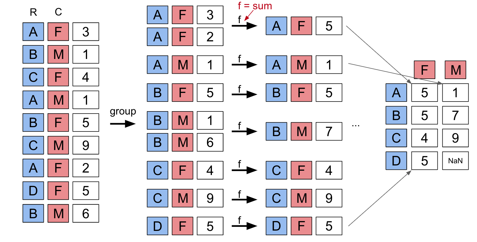
Grouping
Group rows that share a common feature, then aggregate data across the group.
In this example, we count the total number of babies born each year (considering only a small subset of the data for simplicity).
babynames.groupby("Year")
<pandas.core.groupby.generic.DataFrameGroupBy object at 0x7c9731252ad0>
# Grouping by "Year" and aggregating the "Count" column
# to get the total number of babies born each year.
babies_by_year = babynames.groupby("Year")[["Count"]].agg(sum)
babies_by_year
/tmp/ipykernel_273/4059455554.py:3: FutureWarning: The provided callable <built-in function sum> is currently using DataFrameGroupBy.sum. In a future version of pandas, the provided callable will be used directly. To keep current behavior pass the string "sum" instead.
  babies_by_year = babynames.groupby("Year")[["Count"]].agg(sum)
| Count | |
|---|---|
| Year | |
| 1910 | 9163 |
| 1911 | 9983 |
| 1912 | 17946 |
| 1913 | 22094 |
| 1914 | 26926 |
| ... | ... |
| 2018 | 395436 |
| 2019 | 386996 |
| 2020 | 362882 |
| 2021 | 362582 |
| 2022 | 360023 |
113 rows × 1 columns
# Plotting baby counts per year
fig = px.line(babies_by_year, y="Count")
fig.update_layout(font_size=18,
                  autosize=False,
                  width=700,
                  height=400)
Slido Exercise
Try to predict the results of the groupby operation shown. The answer is below the image.

df = pd.DataFrame({
  'col1' : ['A', 'B', 'C', 'A', 'B', 'C', 'A', 'C', 'B'],
  'col2' : [3, 1, 4, 1, 5, 9, 2, 5, 6],
  'col3' : ['ak', 'tx', 'fl', 'hi', 'mi', 'ak', 'ca', 'sd', 'nc']
})
df
| col1 | col2 | col3 | |
|---|---|---|---|
| 0 | A | 3 | ak |
| 1 | B | 1 | tx |
| 2 | C | 4 | fl |
| 3 | A | 1 | hi |
| 4 | B | 5 | mi |
| 5 | C | 9 | ak |
| 6 | A | 2 | ca |
| 7 | C | 5 | sd |
| 8 | B | 6 | nc |
# When we don't specify the columns, pandas will try to apply the aggregation to all columns. See next cell for proof!
df.groupby('col1').agg(max)
/tmp/ipykernel_273/3761652406.py:2: FutureWarning:

The provided callable <built-in function max> is currently using DataFrameGroupBy.max. In a future version of pandas, the provided callable will be used directly. To keep current behavior pass the string "max" instead.
| col2 | col3 | |
|---|---|---|
| col1 | ||
| A | 3 | hi |
| B | 6 | tx |
| C | 9 | sd |
df.groupby('col1')[['col2', 'col3']].agg(max)
/tmp/ipykernel_273/3540046338.py:1: FutureWarning:

The provided callable <built-in function max> is currently using DataFrameGroupBy.max. In a future version of pandas, the provided callable will be used directly. To keep current behavior pass the string "max" instead.
| col2 | col3 | |
|---|---|---|
| col1 | ||
| A | 3 | hi |
| B | 6 | tx |
| C | 9 | sd |
Case Study: Name "Popularity"
In this exercise, let's find the name with sex "F" that has dropped most in popularity since its peak usage in California. We'll start by filtering babynames to only include names corresponding to sex "F".
f_babynames = babynames[babynames["Sex"]=="F"]
f_babynames
| State | Sex | Year | Name | Count | |
|---|---|---|---|---|---|
| 0 | CA | F | 1910 | Mary | 295 |
| 1 | CA | F | 1910 | Helen | 239 |
| 2 | CA | F | 1910 | Dorothy | 220 |
| 3 | CA | F | 1910 | Margaret | 163 |
| 4 | CA | F | 1910 | Frances | 134 |
| ... | ... | ... | ... | ... | ... |
| 239532 | CA | F | 2022 | Zemira | 5 |
| 239533 | CA | F | 2022 | Ziggy | 5 |
| 239534 | CA | F | 2022 | Zimal | 5 |
| 239535 | CA | F | 2022 | Zosia | 5 |
| 239536 | CA | F | 2022 | Zulay | 5 |
239537 rows × 5 columns
To build our intuition on how to answer our research question, let's visualize the prevalence of the name "Jennifer" over time.
jenn_entries = f_babynames[f_babynames["Name"]=="Jennifer"]
jenn_entries
| State | Sex | Year | Name | Count | |
|---|---|---|---|---|---|
| 13610 | CA | F | 1934 | Jennifer | 5 |
| 16325 | CA | F | 1938 | Jennifer | 5 |
| 16993 | CA | F | 1939 | Jennifer | 6 |
| 17533 | CA | F | 1940 | Jennifer | 13 |
| 18210 | CA | F | 1941 | Jennifer | 24 |
| ... | ... | ... | ... | ... | ... |
| 221406 | CA | F | 2018 | Jennifer | 167 |
| 225149 | CA | F | 2019 | Jennifer | 145 |
| 228787 | CA | F | 2020 | Jennifer | 141 |
| 232561 | CA | F | 2021 | Jennifer | 91 |
| 236136 | CA | F | 2022 | Jennifer | 114 |
86 rows × 5 columns
# We'll talk about how to generate plots in a later lecture
fig = px.line(jenn_entries, x="Year", y="Count")

fig.update_layout(font_size = 18,
                  autosize=False,
                  width=1000,
                  height=400)
We'll need a mathematical definition for the change in popularity of a name in California.
Define the metric "Ratio to Peak" (RTP). We'll calculate this as the count of the name in 2022 (the most recent year for which we have data) divided by the largest count of this name in any year.
A demo calculation for Jennifer:
# Construct a Series containing our Jennifer count data
jenn_counts_ser = jenn_entries["Count"]
# In the year with the highest Jennifer count, 6065 Jennifers were born
max_jenn = np.max(jenn_counts_ser)
max_jenn
6065
# Remember that we sorted f_babynames by "Year".
# This means that grabbing the final entry gives us the most recent count of Jennifers: 114
# In 2022, the most recent year for which we have data, 114 Jennifers were born
curr_jenn = jenn_counts_ser.iloc[-1]
curr_jenn
114
# Compute the RTP
curr_jenn / max_jenn
0.018796372629843364
We can also write a function that produces the ratio_to_peakfor a given Series. This will allow us to use .groupby to speed up our computation for all names in the dataset.
def ratio_to_peak(series):
    """
    Compute the RTP for a Series containing the counts per year for a single name (year column sorted ascendingly).
    """
    return series.iloc[-1] / np.max(series)
# Then, find the RTP
ratio_to_peak(jenn_counts_ser)
0.018796372629843364
Now, let's use .groupby to compute the RTPs for all names in the dataset.
You may see a warning message when running the cell below. As discussed in the lecture, pandas can't apply an aggregation function to non-numeric data (it doens't make sense to divide "CA" by a number). We can select numerical columns of interest directly.
rtp_table = f_babynames.groupby("Name")[["Year", "Count"]].agg(ratio_to_peak)
rtp_table
| Year | Count | |
|---|---|---|
| Name | ||
| Aadhini | 1.0 | 1.000000 |
| Aadhira | 1.0 | 0.500000 |
| Aadhya | 1.0 | 0.660000 |
| Aadya | 1.0 | 0.586207 |
| Aahana | 1.0 | 0.269231 |
| ... | ... | ... |
| Zyanya | 1.0 | 0.466667 |
| Zyla | 1.0 | 1.000000 |
| Zylah | 1.0 | 1.000000 |
| Zyra | 1.0 | 1.000000 |
| Zyrah | 1.0 | 0.833333 |
13782 rows × 2 columns
This is the pandas equivalent of .group from Data 8. If we wanted to achieve this same result using the datascience library, we would write:
f_babynames.group("Name", ratio_to_peak)
Slido Exercise
Is there a row where Year is not equal to 1? Recall that babynames is sorted ascending by year.
f_babynames
| State | Sex | Year | Name | Count | |
|---|---|---|---|---|---|
| 0 | CA | F | 1910 | Mary | 295 |
| 1 | CA | F | 1910 | Helen | 239 |
| 2 | CA | F | 1910 | Dorothy | 220 |
| 3 | CA | F | 1910 | Margaret | 163 |
| 4 | CA | F | 1910 | Frances | 134 |
| ... | ... | ... | ... | ... | ... |
| 239532 | CA | F | 2022 | Zemira | 5 |
| 239533 | CA | F | 2022 | Ziggy | 5 |
| 239534 | CA | F | 2022 | Zimal | 5 |
| 239535 | CA | F | 2022 | Zosia | 5 |
| 239536 | CA | F | 2022 | Zulay | 5 |
239537 rows × 5 columns
# Unique values in the Year column
rtp_table["Year"].unique()
array([1.])
A hint: If we randomly shuffle the dataset, we see values of Year other than 1.
- The maximum year for each name is no longer guaranteed to be the last-appearing year for each name! So, the ratio is no longer 1.
f_babynames.sample(frac=1, replace=False).groupby("Name")[["Year", "Count"]].agg(ratio_to_peak)
| Year | Count | |
|---|---|---|
| Name | ||
| Aadhini | 1.000000 | 1.000000 |
| Aadhira | 0.999505 | 0.700000 |
| Aadhya | 0.994560 | 0.160000 |
| Aadya | 0.998516 | 0.793103 |
| Aahana | 0.995054 | 0.653846 |
| ... | ... | ... |
| Zyanya | 0.993076 | 0.666667 |
| Zyla | 1.000000 | 1.000000 |
| Zylah | 0.996044 | 0.642857 |
| Zyra | 0.996538 | 0.437500 |
| Zyrah | 1.000000 | 0.833333 |
13782 rows × 2 columns
# Dropping the "Year" column
rtp_table.drop("Year", axis="columns", inplace=True)
rtp_table
| Count | |
|---|---|
| Name | |
| Aadhini | 1.000000 |
| Aadhira | 0.500000 |
| Aadhya | 0.660000 |
| Aadya | 0.586207 |
| Aahana | 0.269231 |
| ... | ... |
| Zyanya | 0.466667 |
| Zyla | 1.000000 |
| Zylah | 1.000000 |
| Zyra | 1.000000 |
| Zyrah | 0.833333 |
13782 rows × 1 columns
# Rename "Count" to "Count RTP" for clarity
rtp_table = rtp_table.rename(columns={"Count":"Count RTP"})
rtp_table
| Count RTP | |
|---|---|
| Name | |
| Aadhini | 1.000000 |
| Aadhira | 0.500000 |
| Aadhya | 0.660000 |
| Aadya | 0.586207 |
| Aahana | 0.269231 |
| ... | ... |
| Zyanya | 0.466667 |
| Zyla | 1.000000 |
| Zylah | 1.000000 |
| Zyra | 1.000000 |
| Zyrah | 0.833333 |
13782 rows × 1 columns
# What name has fallen the most in popularity?
rtp_table.sort_values("Count RTP")
| Count RTP | |
|---|---|
| Name | |
| Debra | 0.001260 |
| Debbie | 0.002815 |
| Carol | 0.003180 |
| Tammy | 0.003249 |
| Susan | 0.003305 |
| ... | ... |
| Zyla | 1.000000 |
| Zylah | 1.000000 |
| Zyra | 1.000000 |
| Aahna | 1.000000 |
| Aadhini | 1.000000 |
13782 rows × 1 columns
We can visualize the decrease in the popularity of the name "Debra:"
def plot_name(*names):
    fig = px.line(f_babynames[f_babynames["Name"].isin(names)],
                  x="Year", y="Count", color="Name",
                  title=f"Popularity for: {names}")
    fig.update_layout(font_size=18,
                  autosize=False,
                  width=1000,
                  height=400)
    return fig

plot_name("Debra")
# Find the 10 names that have decreased the most in popularity
top10 = rtp_table.sort_values("Count RTP").head(10).index
top10
Index(['Debra', 'Debbie', 'Carol', 'Tammy', 'Susan', 'Cheryl', 'Shannon',
       'Tina', 'Michele', 'Terri'],
      dtype='object', name='Name')
plot_name(*top10)
For fun, try plotting your name or your friends' names.
groupby.size and groupby.count()
df = pd.DataFrame({'letter':['A', 'A', 'B', 'C', 'C', 'C'],
                   'num':[1, 2, 3, 4, np.NaN, 4],
                   'state':[np.NaN, 'tx', 'fl', 'hi', np.NaN, 'ak']})
df
| letter | num | state | |
|---|---|---|---|
| 0 | A | 1.0 | NaN |
| 1 | A | 2.0 | tx |
| 2 | B | 3.0 | fl |
| 3 | C | 4.0 | hi |
| 4 | C | NaN | NaN |
| 5 | C | 4.0 | ak |
groupby.size() returns a Series, indexed by the letters that we grouped by, with values denoting the number of rows in each group/sub-DataFrame. It does not care about missing (NaN) values.
df.groupby("letter").size()
letter
A    2
B    1
C    3
dtype: int64
You might recall value_counts() function we talked about last week. What's the difference?
df["letter"].value_counts()
letter
C    3
A    2
B    1
Name: count, dtype: int64
Turns out value_counts() does something similar to groupby.size(), except that it also sorts the resulting Series in descending order.
groupby.count() returns a DataFrame, indexed by the letters that we grouped by. Each column represents the number of non-missing values for that letter.
df.groupby("letter").count()
| num | state | |
|---|---|---|
| letter | ||
| A | 2 | 1 |
| B | 1 | 1 |
| C | 2 | 2 |
Filtering by Group
Another common use for groups is to filter data:
Usage: groupby(___).filter(func)
.filter() applies func to each group's sub-DataFrame (sf).
funcmust return a scalarTrueorFalsefor eachsf.- If
funcreturnsTruefor asf, then all rows belonging to the group are preserved. - If
funcreturnsFalsefor asf, then all rows belonging to that group are filtered out.
Slido Exercise
Which of the following returns all rows of babynames with names that appeared for the first time after 2010?
babynames.groupby("Name").filter(lambda sf: sf["Year"].min() > 2010)
| State | Sex | Year | Name | Count | |
|---|---|---|---|---|---|
| 195266 | CA | F | 2011 | Mileidy | 15 |
| 195280 | CA | F | 2011 | Solara | 15 |
| 195370 | CA | F | 2011 | Yorley | 14 |
| 195705 | CA | F | 2011 | Mileydi | 11 |
| 195832 | CA | F | 2011 | Kensie | 10 |
| ... | ... | ... | ... | ... | ... |
| 407420 | CA | M | 2022 | Zae | 5 |
| 407421 | CA | M | 2022 | Zai | 5 |
| 407422 | CA | M | 2022 | Zay | 5 |
| 407423 | CA | M | 2022 | Zayvier | 5 |
| 407427 | CA | M | 2022 | Zylo | 5 |
7691 rows × 5 columns
babynames.groupby("Name").filter(lambda sf: sf["Year"].max() > 2010)
| State | Sex | Year | Name | Count | |
|---|---|---|---|---|---|
| 0 | CA | F | 1910 | Mary | 295 |
| 1 | CA | F | 1910 | Helen | 239 |
| 2 | CA | F | 1910 | Dorothy | 220 |
| 3 | CA | F | 1910 | Margaret | 163 |
| 4 | CA | F | 1910 | Frances | 134 |
| ... | ... | ... | ... | ... | ... |
| 407423 | CA | M | 2022 | Zayvier | 5 |
| 407424 | CA | M | 2022 | Zia | 5 |
| 407425 | CA | M | 2022 | Zora | 5 |
| 407426 | CA | M | 2022 | Zuriel | 5 |
| 407427 | CA | M | 2022 | Zylo | 5 |
339263 rows × 5 columns
babynames.groupby("Name").filter(lambda sf: sf["Year"] > 2010)
---------------------------------------------------------------------------
TypeError                                 Traceback (most recent call last)
Cell In[34], line 1
----> 1 babynames.groupby("Name").filter(lambda sf: sf["Year"] > 2010)

File /srv/conda/envs/notebook/lib/python3.11/site-packages/pandas/core/groupby/generic.py:1932, in DataFrameGroupBy.filter(self, func, dropna, *args, **kwargs)
   1929             indices.append(self._get_index(name))
   1930     else:
   1931         # non scalars aren't allowed
-> 1932         raise TypeError(
   1933             f"filter function returned a {type(res).__name__}, "
   1934             "but expected a scalar bool"
   1935         )
   1937 return self._apply_filter(indices, dropna)

TypeError: filter function returned a Series, but expected a scalar bool
babynames.groupby(["Name", "Year"]).filter(lambda sf: sf["Year"] > 2010)
---------------------------------------------------------------------------
TypeError                                 Traceback (most recent call last)
Cell In[35], line 1
----> 1 babynames.groupby(["Name", "Year"]).filter(lambda sf: sf["Year"] > 2010)

File /srv/conda/envs/notebook/lib/python3.11/site-packages/pandas/core/groupby/generic.py:1932, in DataFrameGroupBy.filter(self, func, dropna, *args, **kwargs)
   1929             indices.append(self._get_index(name))
   1930     else:
   1931         # non scalars aren't allowed
-> 1932         raise TypeError(
   1933             f"filter function returned a {type(res).__name__}, "
   1934             "but expected a scalar bool"
   1935         )
   1937 return self._apply_filter(indices, dropna)

TypeError: filter function returned a Series, but expected a scalar bool
# Let's read the elections dataset
elections = pd.read_csv("data/elections.csv")
elections.sample(5)
| Year | Candidate | Party | Popular vote | Result | % | |
|---|---|---|---|---|---|---|
| 171 | 2012 | Mitt Romney | Republican | 60933504 | loss | 47.384076 |
| 118 | 1972 | George McGovern | Democratic | 29173222 | loss | 37.670670 |
| 125 | 1976 | Roger MacBride | Libertarian | 172557 | loss | 0.212451 |
| 55 | 1900 | William Jennings Bryan | Democratic | 6370932 | loss | 46.130540 |
| 142 | 1992 | George H. W. Bush | Republican | 39104550 | loss | 37.544784 |
Let's keep only the elections years where the maximum vote share % is less than 45%.
elections.groupby("Year").filter(lambda sf: sf["%"].max() < 45).head(10)
| Year | Candidate | Party | Popular vote | Result | % | |
|---|---|---|---|---|---|---|
| 23 | 1860 | Abraham Lincoln | Republican | 1855993 | win | 39.699408 |
| 24 | 1860 | John Bell | Constitutional Union | 590901 | loss | 12.639283 |
| 25 | 1860 | John C. Breckinridge | Southern Democratic | 848019 | loss | 18.138998 |
| 26 | 1860 | Stephen A. Douglas | Northern Democratic | 1380202 | loss | 29.522311 |
| 66 | 1912 | Eugene V. Debs | Socialist | 901551 | loss | 6.004354 |
| 67 | 1912 | Eugene W. Chafin | Prohibition | 208156 | loss | 1.386325 |
| 68 | 1912 | Theodore Roosevelt | Progressive | 4122721 | loss | 27.457433 |
| 69 | 1912 | William Taft | Republican | 3486242 | loss | 23.218466 |
| 70 | 1912 | Woodrow Wilson | Democratic | 6296284 | win | 41.933422 |
| 115 | 1968 | George Wallace | American Independent | 9901118 | loss | 13.571218 |
# Why did we get a DataFrame instead of a Series?
# Notice that "%" is in its own sublist!
elections_max_percentage = elections.groupby("Year")[["%"]].agg(max)
elections_max_percentage
/tmp/ipykernel_273/3570771099.py:3: FutureWarning:

The provided callable <built-in function max> is currently using DataFrameGroupBy.max. In a future version of pandas, the provided callable will be used directly. To keep current behavior pass the string "max" instead.
| % | |
|---|---|
| Year | |
| 1824 | 57.210122 |
| 1828 | 56.203927 |
| 1832 | 54.574789 |
| 1836 | 52.272472 |
| 1840 | 53.051213 |
| 1844 | 50.749477 |
| 1848 | 47.309296 |
| 1852 | 51.013168 |
| 1856 | 45.306080 |
| 1860 | 39.699408 |
| 1864 | 54.951512 |
| 1868 | 52.665305 |
| 1872 | 55.928594 |
| 1876 | 51.528376 |
| 1880 | 48.369234 |
| 1884 | 48.884933 |
| 1888 | 48.656799 |
| 1892 | 46.121393 |
| 1896 | 51.213817 |
| 1900 | 52.342640 |
| 1904 | 56.562787 |
| 1908 | 52.013300 |
| 1912 | 41.933422 |
| 1916 | 49.367987 |
| 1920 | 60.574501 |
| 1924 | 54.329113 |
| 1928 | 58.368524 |
| 1932 | 57.672125 |
| 1936 | 60.978107 |
| 1940 | 54.871202 |
| 1944 | 53.773801 |
| 1948 | 49.601536 |
| 1952 | 55.325173 |
| 1956 | 57.650654 |
| 1960 | 50.082561 |
| 1964 | 61.344703 |
| 1968 | 43.565246 |
| 1972 | 60.907806 |
| 1976 | 50.271900 |
| 1980 | 50.897944 |
| 1984 | 59.023326 |
| 1988 | 53.518845 |
| 1992 | 43.118485 |
| 1996 | 49.296938 |
| 2000 | 48.491813 |
| 2004 | 50.771824 |
| 2008 | 53.023510 |
| 2012 | 51.258484 |
| 2016 | 48.521539 |
| 2020 | 51.311515 |
| 2024 | 49.808629 |
elections_max_percentage.sort_values(by="%").head()
| % | |
|---|---|
| Year | |
| 1860 | 39.699408 |
| 1912 | 41.933422 |
| 1992 | 43.118485 |
| 1968 | 43.565246 |
| 1856 | 45.306080 |
groupby Puzzle
Assume that we want to know the best election by each party.
Attempt #1
We have to be careful when using aggregation functions. For example, the code below might be misinterpreted to say that Woodrow Wilson successfully ran for election in 2020. Why is this happening?
elections.groupby("Party").agg(max).head(10)
/tmp/ipykernel_273/4278286395.py:1: FutureWarning:

The provided callable <built-in function max> is currently using DataFrameGroupBy.max. In a future version of pandas, the provided callable will be used directly. To keep current behavior pass the string "max" instead.
| Year | Candidate | Popular vote | Result | % | |
|---|---|---|---|---|---|
| Party | |||||
| American | 1976 | Thomas J. Anderson | 873053 | loss | 21.554001 |
| American Independent | 1976 | Lester Maddox | 9901118 | loss | 13.571218 |
| Anti-Masonic | 1832 | William Wirt | 100715 | loss | 7.821583 |
| Anti-Monopoly | 1884 | Benjamin Butler | 134294 | loss | 1.335838 |
| Citizens | 1980 | Barry Commoner | 233052 | loss | 0.270182 |
| Communist | 1932 | William Z. Foster | 103307 | loss | 0.261069 |
| Constitution | 2016 | Michael Peroutka | 203091 | loss | 0.152398 |
| Constitutional Union | 1860 | John Bell | 590901 | loss | 12.639283 |
| Democratic | 2024 | Woodrow Wilson | 81268924 | win | 61.344703 |
| Democratic-Republican | 1824 | John Quincy Adams | 151271 | win | 57.210122 |
It's generally a good idea to be explicit about which columns to aggregate!
Attempt #2
Next, we'll write code that properly returns the best result by each party. That is, each row should show the Year, Candidate, Popular Vote, Result, and % for the election in which that party saw its best results (rather than mixing them as in the example above). Here's what the first rows of the correct output should look like:

elections_sorted_by_percent = elections.sort_values("%", ascending=False)
elections_sorted_by_percent.head(8)
| Year | Candidate | Party | Popular vote | Result | % | |
|---|---|---|---|---|---|---|
| 114 | 1964 | Lyndon Johnson | Democratic | 43127041 | win | 61.344703 |
| 91 | 1936 | Franklin Roosevelt | Democratic | 27752648 | win | 60.978107 |
| 120 | 1972 | Richard Nixon | Republican | 47168710 | win | 60.907806 |
| 79 | 1920 | Warren Harding | Republican | 16144093 | win | 60.574501 |
| 133 | 1984 | Ronald Reagan | Republican | 54455472 | win | 59.023326 |
| 84 | 1928 | Herbert Hoover | Republican | 21427123 | win | 58.368524 |
| 86 | 1932 | Franklin Roosevelt | Democratic | 22821277 | win | 57.672125 |
| 109 | 1956 | Dwight Eisenhower | Republican | 35579180 | win | 57.650654 |
elections_sorted_by_percent.groupby("Party").first()
| Year | Candidate | Popular vote | Result | % | |
|---|---|---|---|---|---|
| Party | |||||
| American | 1856 | Millard Fillmore | 873053 | loss | 21.554001 |
| American Independent | 1968 | George Wallace | 9901118 | loss | 13.571218 |
| Anti-Masonic | 1832 | William Wirt | 100715 | loss | 7.821583 |
| Anti-Monopoly | 1884 | Benjamin Butler | 134294 | loss | 1.335838 |
| Citizens | 1980 | Barry Commoner | 233052 | loss | 0.270182 |
| Communist | 1932 | William Z. Foster | 103307 | loss | 0.261069 |
| Constitution | 2008 | Chuck Baldwin | 199750 | loss | 0.152398 |
| Constitutional Union | 1860 | John Bell | 590901 | loss | 12.639283 |
| Democratic | 1964 | Lyndon Johnson | 43127041 | win | 61.344703 |
| Democratic-Republican | 1824 | Andrew Jackson | 151271 | loss | 57.210122 |
| Dixiecrat | 1948 | Strom Thurmond | 1175930 | loss | 2.412304 |
| Farmer–Labor | 1920 | Parley P. Christensen | 265398 | loss | 0.995804 |
| Free Soil | 1848 | Martin Van Buren | 291501 | loss | 10.138474 |
| Green | 2000 | Ralph Nader | 2882955 | loss | 2.741176 |
| Greenback | 1880 | James B. Weaver | 308649 | loss | 3.352344 |
| Independent | 1992 | Ross Perot | 19743821 | loss | 18.956298 |
| Liberal Republican | 1872 | Horace Greeley | 2834761 | loss | 44.071406 |
| Libertarian | 2016 | Gary Johnson | 4489235 | loss | 3.307714 |
| Libertarian Party | 2024 | Chase Oliver | 650130 | loss | 0.418895 |
| National Democratic | 1896 | John M. Palmer | 134645 | loss | 0.969566 |
| National Republican | 1828 | John Quincy Adams | 500897 | loss | 43.796073 |
| National Union | 1864 | Abraham Lincoln | 2211317 | win | 54.951512 |
| Natural Law | 1996 | John Hagelin | 113670 | loss | 0.118219 |
| New Alliance | 1988 | Lenora Fulani | 217221 | loss | 0.237804 |
| Northern Democratic | 1860 | Stephen A. Douglas | 1380202 | loss | 29.522311 |
| Populist | 1892 | James B. Weaver | 1041028 | loss | 8.645038 |
| Progressive | 1912 | Theodore Roosevelt | 4122721 | loss | 27.457433 |
| Prohibition | 1892 | John Bidwell | 270879 | loss | 2.249468 |
| Reform | 1996 | Ross Perot | 8085294 | loss | 8.408844 |
| Republican | 1972 | Richard Nixon | 47168710 | win | 60.907806 |
| Socialist | 1912 | Eugene V. Debs | 901551 | loss | 6.004354 |
| Southern Democratic | 1860 | John C. Breckinridge | 848019 | loss | 18.138998 |
| States' Rights | 1956 | T. Coleman Andrews | 107929 | loss | 0.174883 |
| Taxpayers | 1996 | Howard Phillips | 184656 | loss | 0.192045 |
| Union | 1936 | William Lemke | 892378 | loss | 1.960733 |
| Union Labor | 1888 | Alson Streeter | 146602 | loss | 1.288861 |
| Whig | 1840 | William Henry Harrison | 1275583 | win | 53.051213 |
Alternative Solutions
You'll soon discover that with Pandas rich tool set, there's typically more than one way to get to the same answer. Each approach has different tradeoffs in terms of readability, performance, memory consumption, complexity, and more. It will take some experience for you to develop a sense of which approach is better for each problem, but you should, in general, try to think if you can at least envision a different solution to a given problem, especially if you find your current solution to be particularly convoluted or hard to read.
Here are a couple of other ways of obtaining the same result (in each case, we only show the top part with head()). The first approach uses groupby but finds the location of the maximum value via the idxmax() method (look up its documentation!). We then index and sort by Party to match the requested formatting:
elections.groupby("Party")["%"].idxmax()
Party
American                  22
American Independent     115
Anti-Masonic               6
Anti-Monopoly             38
Citizens                 127
Communist                 89
Constitution             164
Constitutional Union      24
Democratic               114
Democratic-Republican      0
Dixiecrat                103
Farmer–Labor              78
Free Soil                 15
Green                    155
Greenback                 35
Independent              143
Liberal Republican        31
Libertarian              175
Libertarian Party        186
National Democratic       50
National Republican        3
National Union            27
Natural Law              148
New Alliance             136
Northern Democratic       26
Populist                  48
Progressive               68
Prohibition               49
Reform                   150
Republican               120
Socialist                 66
Southern Democratic       25
States' Rights           110
Taxpayers                147
Union                     93
Union Labor               42
Whig                      11
Name: %, dtype: int64
# This is the computational part
best_per_party = elections.loc[elections.groupby("Party")["%"].idxmax()]

# This indexes by Party to match the formatting above
best_per_party.set_index('Party').sort_index().head()
| Year | Candidate | Popular vote | Result | % | |
|---|---|---|---|---|---|
| Party | |||||
| American | 1856 | Millard Fillmore | 873053 | loss | 21.554001 |
| American Independent | 1968 | George Wallace | 9901118 | loss | 13.571218 |
| Anti-Masonic | 1832 | William Wirt | 100715 | loss | 7.821583 |
| Anti-Monopoly | 1884 | Benjamin Butler | 134294 | loss | 1.335838 |
| Citizens | 1980 | Barry Commoner | 233052 | loss | 0.270182 |
And this one doesn't even use groupby! This approach instead uses the drop_duplicates method to keep only the last occurrence of of each party after having sorted by "%", which is the best performance. Again, the 2nd line is purely formatting:
best_per_party2 = elections.sort_values("%").drop_duplicates(["Party"], keep="last")
best_per_party2.set_index("Party").sort_index().head()  # Formatting
| Year | Candidate | Popular vote | Result | % | |
|---|---|---|---|---|---|
| Party | |||||
| American | 1856 | Millard Fillmore | 873053 | loss | 21.554001 |
| American Independent | 1968 | George Wallace | 9901118 | loss | 13.571218 |
| Anti-Masonic | 1832 | William Wirt | 100715 | loss | 7.821583 |
| Anti-Monopoly | 1884 | Benjamin Butler | 134294 | loss | 1.335838 |
| Citizens | 1980 | Barry Commoner | 233052 | loss | 0.270182 |
Challenge: See if you can find yet another approach that still gives the same answer.
DataFrameGroupBy Objects
The result of groupby is not a DataFrame or a list of DataFrames. It is instead a special type called a DataFrameGroupBy.
grouped_by_party = elections.groupby("Party")
type(grouped_by_party)
pandas.core.groupby.generic.DataFrameGroupBy
GroupBy objects are structured like dictionaries. In fact, we can actually see the dictionaries with the following code:
grouped_by_party.groups
{'American': [22, 126], 'American Independent': [115, 119, 124], 'Anti-Masonic': [6], 'Anti-Monopoly': [38], 'Citizens': [127], 'Communist': [89], 'Constitution': [160, 164, 172], 'Constitutional Union': [24], 'Democratic': [2, 4, 8, 10, 13, 14, 17, 20, 28, 29, 34, 37, 39, 45, 47, 52, 55, 57, 64, 70, 74, 77, 81, 83, 86, 91, 94, 97, 100, 105, 108, 111, 114, 116, 118, 123, 129, 134, 137, 140, 144, 151, 158, 162, 168, 176, 178, 183], 'Democratic-Republican': [0, 1], 'Dixiecrat': [103], 'Farmer–Labor': [78], 'Free Soil': [15, 18], 'Green': [149, 155, 156, 165, 170, 177, 181, 184], 'Greenback': [35], 'Independent': [121, 130, 143, 161, 167, 174, 185], 'Liberal Republican': [31], 'Libertarian': [125, 128, 132, 138, 139, 146, 153, 159, 163, 169, 175, 180], 'Libertarian Party': [186], 'National Democratic': [50], 'National Republican': [3, 5], 'National Union': [27], 'Natural Law': [148], 'New Alliance': [136], 'Northern Democratic': [26], 'Populist': [48, 61, 141], 'Progressive': [68, 82, 101, 107], 'Prohibition': [41, 44, 49, 51, 54, 59, 63, 67, 73, 75, 99], 'Reform': [150, 154], 'Republican': [21, 23, 30, 32, 33, 36, 40, 43, 46, 53, 56, 60, 65, 69, 72, 79, 80, 84, 87, 90, 96, 98, 104, 106, 109, 112, 113, 117, 120, 122, 131, 133, 135, 142, 145, 152, 157, 166, 171, 173, 179, 182], 'Socialist': [58, 62, 66, 71, 76, 85, 88, 92, 95, 102], 'Southern Democratic': [25], 'States' Rights': [110], 'Taxpayers': [147], 'Union': [93], 'Union Labor': [42], 'Whig': [7, 9, 11, 12, 16, 19]}
The keys of the dictionary are the groups (in this case, Party), and the values are the indices of rows belonging to that group. We can access a particular sub-DataFrame using get_group:
grouped_by_party.get_group("Socialist")
| Year | Candidate | Party | Popular vote | Result | % | |
|---|---|---|---|---|---|---|
| 58 | 1904 | Eugene V. Debs | Socialist | 402810 | loss | 2.985897 |
| 62 | 1908 | Eugene V. Debs | Socialist | 420852 | loss | 2.850866 |
| 66 | 1912 | Eugene V. Debs | Socialist | 901551 | loss | 6.004354 |
| 71 | 1916 | Allan L. Benson | Socialist | 590524 | loss | 3.194193 |
| 76 | 1920 | Eugene V. Debs | Socialist | 913693 | loss | 3.428282 |
| 85 | 1928 | Norman Thomas | Socialist | 267478 | loss | 0.728623 |
| 88 | 1932 | Norman Thomas | Socialist | 884885 | loss | 2.236211 |
| 92 | 1936 | Norman Thomas | Socialist | 187910 | loss | 0.412876 |
| 95 | 1940 | Norman Thomas | Socialist | 116599 | loss | 0.234237 |
| 102 | 1948 | Norman Thomas | Socialist | 139569 | loss | 0.286312 |
Pivot Tables
Groupby with multiple columns
We want to build a table showing the total number of babies born of each sex in each year. One way is to groupby using both columns of interest:
babynames.groupby(["Year", "Sex"])[["Count"]].sum().head(6)
| Count | ||
|---|---|---|
| Year | Sex | |
| 1910 | F | 5950 |
| M | 3213 | |
| 1911 | F | 6602 |
| M | 3381 | |
| 1912 | F | 9804 |
| M | 8142 |
pivot_table
babynames.pivot_table(
    index="Year",
    columns="Sex",
    values="Count",
    aggfunc=np.sum).head(6)
/tmp/ipykernel_273/3588306476.py:1: FutureWarning:

The provided callable <function sum at 0x7c975ce83740> is currently using DataFrameGroupBy.sum. In a future version of pandas, the provided callable will be used directly. To keep current behavior pass the string "sum" instead.
| Sex | F | M |
|---|---|---|
| Year | ||
| 1910 | 5950 | 3213 |
| 1911 | 6602 | 3381 |
| 1912 | 9804 | 8142 |
| 1913 | 11860 | 10234 |
| 1914 | 13815 | 13111 |
| 1915 | 18643 | 17192 |
pivot_table with Multiple values
babynames.pivot_table(
    index="Year",
    columns="Sex",
    values=["Count", "Name"],
    aggfunc=np.max).head(6)
/tmp/ipykernel_273/3274469386.py:1: FutureWarning:

The provided callable <function max at 0x7c975ce83e20> is currently using DataFrameGroupBy.max. In a future version of pandas, the provided callable will be used directly. To keep current behavior pass the string "max" instead.
| Count | Name | |||
|---|---|---|---|---|
| Sex | F | M | F | M |
| Year | ||||
| 1910 | 295 | 237 | Yvonne | William |
| 1911 | 390 | 214 | Zelma | Willis |
| 1912 | 534 | 501 | Yvonne | Woodrow |
| 1913 | 584 | 614 | Zelma | Yoshio |
| 1914 | 773 | 769 | Zelma | Yoshio |
| 1915 | 998 | 1033 | Zita | Yukio |
Join Tables
What if we want to know the popularity of presidential candidates' first names in California in 2022? What can we do?
elections.head(10)
| Year | Candidate | Party | Popular vote | Result | % | |
|---|---|---|---|---|---|---|
| 0 | 1824 | Andrew Jackson | Democratic-Republican | 151271 | loss | 57.210122 |
| 1 | 1824 | John Quincy Adams | Democratic-Republican | 113142 | win | 42.789878 |
| 2 | 1828 | Andrew Jackson | Democratic | 642806 | win | 56.203927 |
| 3 | 1828 | John Quincy Adams | National Republican | 500897 | loss | 43.796073 |
| 4 | 1832 | Andrew Jackson | Democratic | 702735 | win | 54.574789 |
| 5 | 1832 | Henry Clay | National Republican | 484205 | loss | 37.603628 |
| 6 | 1832 | William Wirt | Anti-Masonic | 100715 | loss | 7.821583 |
| 7 | 1836 | Hugh Lawson White | Whig | 146109 | loss | 10.005985 |
| 8 | 1836 | Martin Van Buren | Democratic | 763291 | win | 52.272472 |
| 9 | 1836 | William Henry Harrison | Whig | 550816 | loss | 37.721543 |
babynames_2022 = babynames[babynames["Year"]==2022]
babynames_2022.head(10)
| State | Sex | Year | Name | Count | |
|---|---|---|---|---|---|
| 235835 | CA | F | 2022 | Olivia | 2178 |
| 235836 | CA | F | 2022 | Emma | 2080 |
| 235837 | CA | F | 2022 | Camila | 2046 |
| 235838 | CA | F | 2022 | Mia | 1882 |
| 235839 | CA | F | 2022 | Sophia | 1762 |
| 235840 | CA | F | 2022 | Isabella | 1733 |
| 235841 | CA | F | 2022 | Luna | 1516 |
| 235842 | CA | F | 2022 | Sofia | 1307 |
| 235843 | CA | F | 2022 | Amelia | 1289 |
| 235844 | CA | F | 2022 | Gianna | 1107 |
elections["First Name"] = elections["Candidate"].str.split(" ").str[0]
elections
| Year | Candidate | Party | Popular vote | Result | % | First Name | |
|---|---|---|---|---|---|---|---|
| 0 | 1824 | Andrew Jackson | Democratic-Republican | 151271 | loss | 57.210122 | Andrew |
| 1 | 1824 | John Quincy Adams | Democratic-Republican | 113142 | win | 42.789878 | John |
| 2 | 1828 | Andrew Jackson | Democratic | 642806 | win | 56.203927 | Andrew |
| 3 | 1828 | John Quincy Adams | National Republican | 500897 | loss | 43.796073 | John |
| 4 | 1832 | Andrew Jackson | Democratic | 702735 | win | 54.574789 | Andrew |
| ... | ... | ... | ... | ... | ... | ... | ... |
| 182 | 2024 | Donald Trump | Republican | 77303568 | win | 49.808629 | Donald |
| 183 | 2024 | Kamala Harris | Democratic | 75019230 | loss | 48.336772 | Kamala |
| 184 | 2024 | Jill Stein | Green | 861155 | loss | 0.554864 | Jill |
| 185 | 2024 | Robert Kennedy | Independent | 756383 | loss | 0.487357 | Robert |
| 186 | 2024 | Chase Oliver | Libertarian Party | 650130 | loss | 0.418895 | Chase |
187 rows × 7 columns
Unlike in Data 8, the join function is called merge in pandas. join in pandas does something slightly different—we won't talk about it in this class.
merged = pd.merge(left=elections, right=babynames_2022,
                  left_on="First Name", right_on="Name")
merged
| Year_x | Candidate | Party | Popular vote | Result | % | First Name | State | Sex | Year_y | Name | Count | |
|---|---|---|---|---|---|---|---|---|---|---|---|---|
| 0 | 1824 | Andrew Jackson | Democratic-Republican | 151271 | loss | 57.210122 | Andrew | CA | M | 2022 | Andrew | 741 |
| 1 | 1824 | John Quincy Adams | Democratic-Republican | 113142 | win | 42.789878 | John | CA | M | 2022 | John | 490 |
| 2 | 1828 | Andrew Jackson | Democratic | 642806 | win | 56.203927 | Andrew | CA | M | 2022 | Andrew | 741 |
| 3 | 1828 | John Quincy Adams | National Republican | 500897 | loss | 43.796073 | John | CA | M | 2022 | John | 490 |
| 4 | 1832 | Andrew Jackson | Democratic | 702735 | win | 54.574789 | Andrew | CA | M | 2022 | Andrew | 741 |
| ... | ... | ... | ... | ... | ... | ... | ... | ... | ... | ... | ... | ... |
| 151 | 2020 | Howard Hawkins | Green | 405035 | loss | 0.255731 | Howard | CA | M | 2022 | Howard | 18 |
| 152 | 2024 | Donald Trump | Republican | 77303568 | win | 49.808629 | Donald | CA | M | 2022 | Donald | 33 |
| 153 | 2024 | Robert Kennedy | Independent | 756383 | loss | 0.487357 | Robert | CA | M | 2022 | Robert | 404 |
| 154 | 2024 | Chase Oliver | Libertarian Party | 650130 | loss | 0.418895 | Chase | CA | F | 2022 | Chase | 6 |
| 155 | 2024 | Chase Oliver | Libertarian Party | 650130 | loss | 0.418895 | Chase | CA | M | 2022 | Chase | 203 |
156 rows × 12 columns
merged.sort_values("Count", ascending=False)
| Year_x | Candidate | Party | Popular vote | Result | % | First Name | State | Sex | Year_y | Name | Count | |
|---|---|---|---|---|---|---|---|---|---|---|---|---|
| 36 | 1884 | Benjamin Butler | Anti-Monopoly | 134294 | loss | 1.335838 | Benjamin | CA | M | 2022 | Benjamin | 1524 |
| 40 | 1888 | Benjamin Harrison | Republican | 5443633 | win | 47.858041 | Benjamin | CA | M | 2022 | Benjamin | 1524 |
| 42 | 1892 | Benjamin Harrison | Republican | 5176108 | loss | 42.984101 | Benjamin | CA | M | 2022 | Benjamin | 1524 |
| 21 | 1856 | James Buchanan | Democratic | 1835140 | win | 45.306080 | James | CA | M | 2022 | James | 1086 |
| 35 | 1880 | James Garfield | Republican | 4453337 | win | 48.369234 | James | CA | M | 2022 | James | 1086 |
| ... | ... | ... | ... | ... | ... | ... | ... | ... | ... | ... | ... | ... |
| 97 | 1964 | Lyndon Johnson | Democratic | 43127041 | win | 61.344703 | Lyndon | CA | M | 2022 | Lyndon | 6 |
| 69 | 1916 | Woodrow Wilson | Democratic | 9126868 | win | 49.367987 | Woodrow | CA | M | 2022 | Woodrow | 6 |
| 41 | 1888 | Clinton B. Fisk | Prohibition | 249819 | loss | 2.196299 | Clinton | CA | M | 2022 | Clinton | 6 |
| 154 | 2024 | Chase Oliver | Libertarian Party | 650130 | loss | 0.418895 | Chase | CA | F | 2022 | Chase | 6 |
| 143 | 2016 | Darrell Castle | Constitution | 203091 | loss | 0.149640 | Darrell | CA | M | 2022 | Darrell | 5 |
156 rows × 12 columns