data/calls_for_service.csv ======================
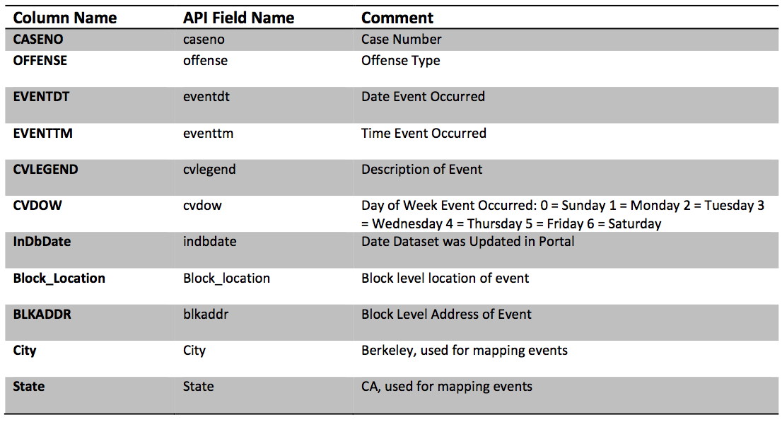
0 'CASENO,OFFENSE,EVENTDT,EVENTTM,CVLEGEND,CVDOW,InDbDate,Block_Location,BLKADDR,City,State\n'
1 '19092769,THEFT MISD. (UNDER $950),12/09/2019 12:00:00 AM,13:00,LARCENY,1,09/10/2020 07:00:11 AM,"SHATTUCK AVE\n'
2 'Berkeley, CA",SHATTUCK AVE,Berkeley,CA\n'
3 '19045891,NARCOTICS,08/18/2019 12:00:00 AM,17:20,DRUG VIOLATION,0,09/10/2020 07:00:08 AM,"FRONTAGE STREET &GILMAN ST\n'
4 'Berkeley, CA",FRONTAGE STREET &GILMAN ST,Berkeley,CA\n'
5 '19060215,ASSAULT/BATTERY MISD.,10/23/2019 12:00:00 AM,10:45,ASSAULT,3,09/10/2020 07:00:10 AM,"2200 MILVIA ST\n'
6 'Berkeley, CA\n'
7 '(37.868574, -122.270415)",2200 MILVIA ST,Berkeley,CA\n'
8 '19092681,VANDALISM,12/01/2019 12:00:00 AM,18:40,VANDALISM,0,09/10/2020 07:00:11 AM,"VIRGINIA ST\n'
9 'Berkeley, CA",VIRGINIA ST,Berkeley,CA\n'
10 '19044228,ASSAULT/BATTERY MISD.,08/10/2019 12:00:00 AM,22:51,ASSAULT,6,09/10/2020 07:00:08 AM,"UNIVERSITY AVENUE &FRONTAGE\n'
11 'Berkeley, CA",UNIVERSITY AVENUE &FRONTAGE,Berkeley,CA\n'
12 '19092551,THEFT MISD. (UNDER $950),11/17/2019 12:00:00 AM,12:00,LARCENY,0,09/10/2020 07:00:11 AM,"ASHBY AVE\n'
13 'Berkeley, CA",ASHBY AVE,Berkeley,CA\n'
14 '19047517,BURGLARY AUTO,08/25/2019 12:00:00 AM,18:25,BURGLARY - VEHICLE,0,09/10/2020 07:00:08 AM,"CATALINA AVE\n'
15 'Berkeley, CA",CATALINA AVE,Berkeley,CA\n'
16 '19091711,VANDALISM,08/19/2019 12:00:00 AM,22:00,VANDALISM,1,09/10/2020 07:00:08 AM,"CALIFORNIA STREET & FAIRVIEW ST\n'
17 'Berkeley, CA",CALIFORNIA STREET & FAIRVIEW ST,Berkeley,CA\n'
18 '19092111,VANDALISM,09/24/2019 12:00:00 AM,20:00,VANDALISM,2,09/10/2020 07:00:09 AM,"600 CANYON RD\n'
19 'Berkeley, CA",600 CANYON RD,Berkeley,CA\n'