import numpy as np
import pandas as pd
import plotly.express as px
import sklearn.linear_model as lm
import seaborn as sns
from tqdm.notebook import tqdm
⏪ Data 8 Review: Bootstrapping, Confidence Intervals, and Hypothesis Testing
Suppose we want to estimate some fixed population-level quantity, like the true average height of all 32,000 UC Berkeley undergraduates. We assume that this true average height is a fixed but unknown quantity. In other words, the population-level statistic is not a random variable.
In a perfect world, we would measure the height of every UC Berkeley undergraduate, calculate the average height, and have a perfect answer to our question. But, cannot reasonably measure the height of every UC Berkeley undergraduate. Instead, we might take a random sample of, say, 10 UC Berkeley students, calculate the sample average, and then use that sample average as our "best guess" of the true average height of all 32,000 UC Berkeley students.
Here's a (fake) random sample of 10 UC Berkeley undergraduate heights in inches, along with the sample mean of those heights:
heights = np.array([68, 67, 69, 66, 66, 66, 71, 72, 61, 70])
heights.mean()
67.6
We would say that 67.6 inches is our "best guess" of the true average height of UC Berkeley undergraduates.
Unlike the true average height, your "best guess" is a random quantity. For example, if you and a friend separately sampled 10 UC Berkeley undergraduates, your sample average heights will probably differ due to randomness in the sample. This begs the question: How much could our "best guesses" differ?
To answer this question, it would be useful for us to measure the variability of our sample statistic across parallel universes of random samples. But, we have another problem: We only get to observe one universe!
In Data 8, you learned that bootstrapping can be used to construct synthetic parallel universes. For example, here's how we could construct synthetic bags of M&Ms from one bag of M&Ms:
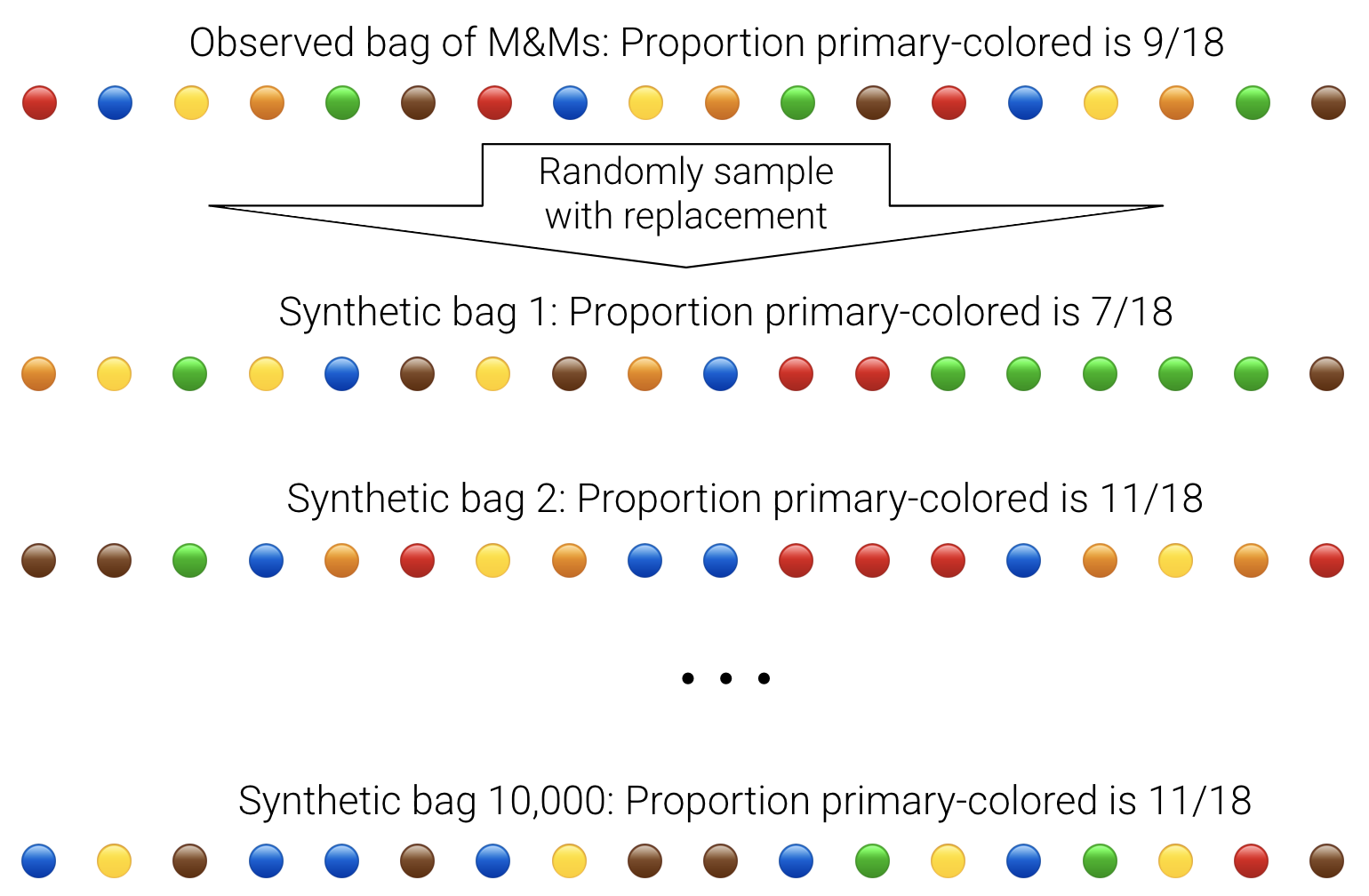
Here are the steps of bootstrapping written out:
- Assume that your random sample of size
nis representative of the true population. - To mimic a random draw of size
nfrom the true population, randomly resamplenobservations with replacement from your random sample. Call this a "synthetic" random sample. - To compute a synthetic "best guess", caculate the sample statistic using your synthetic random sample. For example, you could calculate the sample average.
- Repeat steps 1 and 2 many times. A common choice is 10,000 times.
- The distribution of the 10,000 synthetic "best guesses" provide a sense of uncertainty around your original "best guess".
Here's how we could generate just one synthetic random sample of heights:
# Set seed for reproducibility
np.random.seed(100)
sample_size = len(heights)
# Resample n values with replacement from our real sample of 10 heights
synth_heights = np.random.choice(heights, size=sample_size, replace=True)
# Compute the mean of the synthetic sample
synth_estimate = synth_heights.mean()
print("Original Heights:")
print(heights)
print("Mean of Original Heights:")
print(heights.mean())
print()
print("Synthetic Heights:")
print(synth_heights)
print("Mean of Synthetic Heights:")
print(synth_estimate)
Original Heights: [68 67 69 66 66 66 71 72 61 70] Mean of Original Heights: 67.6 Synthetic Heights: [61 61 66 72 72 68 66 69 66 69] Mean of Synthetic Heights: 67.0
Notice that our synthetic sample mean of 67 inches differs from our original "best guess" of 67.6 inches.
Let's repeat this 10,000 times:
sample_size = len(heights)
n_boot = 10000
# Create an empty array to hold the 10,000 synthetic "best guesses"
synth_estimates = np.zeros(n_boot)
for i in range(n_boot):
# Resample n values with replacement from our real sample of 10 heights
synth_heights = np.random.choice(heights, size=sample_size, replace=True)
# Compute the mean of the synthetic sample
synth_estimate = synth_heights.mean()
# Append the synthetic mean to synth_estimates
synth_estimates[i] = synth_estimate
print('Number of synthetic best guesses:')
print(len(synth_estimates))
print('First 5 synthetic best guesses:')
print(synth_estimates[:5])
Number of synthetic best guesses: 10000 First 5 synthetic best guesses: [67.8 66.9 68.3 67.8 66. ]
To get a sense of how much our best guess could vary across parallel universes, we can visualize the resulting distribution of synthetic best guesses:
fig = px.histogram(pd.Series(synth_estimates),
title='Bootstrap Distribution of the Sample Mean Height',
width=800, histnorm='probability',
barmode="overlay", opacity=0.8)
fig.show()
It looks like the best guesses of most parallel universes fall between 65 inches and 70 inches.
Bootstrap confidence intervals
Suppose a construction manager at Berkeley asked you to find the sample mean height of Berkeley undergraduates so that doors in a new building were not too high or too low. It would be a good idea to not only provide your best guess of 67 inches, but also provide a sense of how uncertain you are about your best guess.
To do so, we can construct and report a bootstrap confidence interval (CI). For example, to construct a 95% CI, we would grab the middle 95% of the synthetic best guesses. In other words, we would grab the 2.5th percentile and the 97.5th percentile:
# Grab the 2.5th and 97.5th percentiles of the synthetic sample means
ci_bounds = np.percentile(synth_estimates, [2.5, 97.5])
print("Lower bound of 95% CI: ", ci_bounds[0])
print("Upper bound of 95% CI: ", ci_bounds[1])
fig.add_vline(x=ci_bounds[0], line_color='red')
fig.add_vline(x=ci_bounds[1], line_color='red')
fig.add_annotation(x=ci_bounds[0], y=0.02, text="Lower Bound", showarrow=True, arrowhead=2)
fig.add_annotation(x=ci_bounds[1], y=0.02, text="Upper Bound", showarrow=True, arrowhead=2)
fig.show()
Lower bound of 95% CI: 65.6 Upper bound of 95% CI: 69.4
Given the values above, we could say "We are 95% confident that the true average height of UC Berkeley undergrads is between 65.6 inches and 69.4 inches."
- What "confidence" really means: Across parallel universes, we think that 95% of our synthetic sample estimates would fall between 65.6 inches and 69.4 inches.
This knowledge of uncertainty around our best guess can help us make better decisions than a single best guess alone.
Bootstrap hypothesis testing
We can also use our confidence interval to perform hypothesis testing. For example, someone might claim that the true average height of UC Berkeley undergrads is 68 inches. This person has proposed what is called a null hypothesis.
$$ \text{Null hypothesis }H_0: \mu = 68, $$
In the definition above, $\mu$ is claimed the true average height of Berkeley undergrads. We can show this null population mean on our plot from above:
fig.add_vline(x=68, line_color='green')
fig.add_annotation(x=68, y=0.02, text="Null population mean", showarrow=True, arrowhead=2)
fig.add_annotation(x=ci_bounds[1], y=0.02, text="Upper Bound", showarrow=True, arrowhead=2)
fig.show()
Our best guess of the true average height based on our original sample is 67.6 inches. But, our bootstrap distribution of the sample mean shows that we could have plausibly made a best guess of 68 inches, in a parallel universe.
Statistical logic (out of scope) tells us to therefore fail to reject the hypothesis that the true average height is 68 inches at a 5% significance level.
- This does not mean that the true average height is exactly 68 inches (i.e., that the hypothesis is true, or that we accept the hypothesis).
- Instead, all we can say is that our sample data could have plausibly been observed if the true average height were indeed 68 inches, so we can't rule out the possibility that the true average height is in fact 68 inches.
- The significance level is calculated by subtracting the confidence level from 1.
If we claimed that the true average height were, say, 70 inches, then we would reject the null hypothesis at the 5% level, since 70 inches falls outside of our 95% confidence interval.
- In other words, it is unlikely that we could have observed a sample average height of 70 inches in a parallel universe.
From last lecture: Bias, variance, and MSE of an estimator
In the last lecture, we learned about the bias, variance, and MSE of an estimator, which are composed of expectations over infinite possible random samples of the data:
$$ \text{Bias}(\hat{\theta}) = \mathbb{E} \left[ \hat{\theta} \right] - \theta $$
$$ \text{Variance}(\hat{\theta}) = \mathbb{E}\left[ \left( \hat{\theta} - \mathbb{E}(\hat{\theta}) \right)^2 \right] $$
$$ \text{MSE}(\hat{\theta}) = \mathbb{E}\left[ \left( \hat{\theta} - \theta \right)^2 \right] $$
Notice that the variance formula does not require us to know $\theta$. So, we can estimate the variance of our estimator using the bootstrap distribution of $\hat{\theta}$'s.
Estimating variance is an important component of constructing normally-approximated bootstrapped confidence intervals, which are beyond the scope of Data 100.
To estimate expectation from a random sample of B synthetic values of $\hat{\theta}$, we just compute the sample mean of the $\hat{\theta}$'s:
$$ \widehat{\mathbb{E}(\hat{\theta})} = \text{Sample mean of }\hat{\theta}\text{'s} = \bar{\hat{\theta}} = \frac{1}{B} \sum_{i=1}^B \hat{\theta}_i $$
To estimate variance from a random sample of B synthetic values of $\hat{\theta}$, we just compute the sample variance of the $\hat{\theta}$'s:
$$ \widehat{\text{Var}(\hat{\theta})} = \text{Sample variance of }\hat{\theta}\text{'s} \approx \frac{1}{B} \sum_{i=1}^B (\hat{\theta}_i - \bar{\hat{\theta}} )^2 $$
The $\approx$ above is out of scope for Data 100. Don't worry about it!
# Estimate expectation using a mean:
estimated_expectation_theta_hat = synth_estimates.mean()
# Same idea for estimated variance
estimated_variance_theta_hat = np.mean((synth_estimates - estimated_expectation_theta_hat) ** 2)
print("Estimated variance of the synthetic sample means: ", estimated_variance_theta_hat)
Estimated variance of the synthetic sample means: 0.9209339375
# np.var directly computes the variance of an array, so we get the same answer!
sample_variance_est = np.var(synth_estimates)
print("Estimated variance of the synthetic sample means: ", sample_variance_est)
Estimated variance of the synthetic sample means: 0.9209339375
Important Data 100 skill from this section: Understand how population level quantities like $\mathbb{E}(\text{Something})$ and $\text{Var}(\text{Something})$ can be estimated with a sample of $\text{Something}_i$'s.
Instructor note: Return to slides!
🍝 Bootstrapping a regression coefficient
For demonstration, we will fit an SLR model to a random sample of the mpg dataset predicting mpg (miles per gallon) from the weight (weight of the vehicle):
$$ \widehat{\text{mpg}} = \hat{\theta}_0 + \hat{\theta}_1 * \text{weight} $$
Then, using the bootstrap, we will construct a confidence interval around the $\hat{\theta}_1$ coefficient.
- This confidence interval tells us the values of $\hat{\theta}_1$ that we could have observed in a parallel universe where a different random sample of cars of the same size were selected.
Suppose we collected a simple random sample of 20 cars from a population of cars. For the purposes of this demo we will assume that seaborn's mpg dataset is the population of all cars.
Here's a visualization of our sample and SLR model:
# Set seed for reproducibility
np.random.seed(42)
# Number of cars to sample
sample_size = 20
# Load in the mpg from seaborn
mpg = sns.load_dataset('mpg')
print("Full Data Size:", len(mpg))
# Sample `sample_size` rows from the mpg dataset
mpg_sample = mpg.sample(sample_size)
print("Sample Size:", len(mpg_sample))
px.scatter(mpg_sample, x='weight', y='mpg', trendline='ols', width=800)
Full Data Size: 398 Sample Size: 20
We can fit linear model with sklearn to get an estimate of the slope:
model = lm.LinearRegression().fit(mpg_sample[['weight']], mpg_sample['mpg'])
print("Slope of the regression line: ", model.coef_[0])
print("Intercept of the regression line: ", model.intercept_)
Slope of the regression line: -0.0069218218719096815 Intercept of the regression line: 43.529512519963816
Our "best guess" of the estimated increase in mpg associated with a one-unit increase in weight is -0.007.
But, best guess is not the end of the story! We can use the bootstrap to measure uncertainty around our best guess.
Bootstrap Implementation
Now let's use the bootstrap to estimate what $\hat{\theta}_1$ might look like across parallel universes of SLR models fit to different random samples.
To make our code reusable, let's write a bootstrap function that takes in a random sample and an estimator function (i.e., the sample mean or a function to extract the $\hat{\theta}_1$ coefficient from an SLR), and then uses that estimator function to construct many synthetic estimates.
def estimator(sample):
"""
Fits an SLR to `sample` regressing mpg on weight,
and returns the slope of the fitted line
"""
model = lm.LinearRegression().fit(sample[['weight']], sample['mpg'])
return (model.intercept_, model.coef_[0])
estimator(mpg_sample)
(43.529512519963816, -0.0069218218719096815)
As expected, our estimator function returns the same intercept and slope as the model we fit above, so long as we plug in the original sample of cars.
print("Slope of the regression line: ", model.coef_[0])
print("Intercept of the regression line: ", model.intercept_)
Slope of the regression line: -0.0069218218719096815 Intercept of the regression line: 43.529512519963816
Next, we will write the general-purpose bootstrap function.
Writing a general-purpose bootstrap function is a very classic problem. It could show up in an interview or on-the-job. Good to understand this section well!
The bootstrap function code uses df.sample (link) to generate a bootstrap sample of the same size of the original sample.
def bootstrap(sample, statistic, num_repetitions):
"""
Returns the statistic computed on a num_repetitions
bootstrap samples from sample.
"""
stats = []
# tqdm provides a progress bar
# functionally, this code is the same as `for i in np.arange(num_repetitions)`
for i in tqdm(np.arange(num_repetitions), "Bootstrapping"):
# Step 1: Resample with replacement from our original sample to generate
# a synthetic sample of the same size
bootstrap_sample = sample.sample(frac=1, replace=True)
# Step 2: Calculate a synthetic estimate using the synthetic sample
bootstrap_stat = statistic(bootstrap_sample)
# Append the synthetic estimate to the list of estimates
stats.append(bootstrap_stat)
return stats
Constructing MANY bootstrap slope estimates:
In general,
10,000is a good default for the number of synthetic samples to compute. In this case, we will use1,000just so our code runs a little faster.
bs_thetas = bootstrap(mpg_sample, estimator, 1000)
print("Number of bootstrap estimates:", len(bs_thetas))
print("First 5 bootstrap estimates:", bs_thetas[:5])
Bootstrapping: 0%| | 0/1000 [00:00<?, ?it/s]
Number of bootstrap estimates: 1000 First 5 bootstrap estimates: [(43.215970007392926, -0.006714853868176342), (45.26126846596228, -0.007064625623981777), (46.602470109629174, -0.007653151422012398), (45.84303440370839, -0.007484470553621759), (46.17677039482411, -0.007577745379669565)]
We can visualize the 1,000 synthetic SLR models we fit with the bootstrap:
# Plot the SLR models given in bs_thetas
# Create a DataFrame from the list of tuples
# Make a scatterplot of the original data
fig = px.scatter(mpg_sample, x='weight', y='mpg', trendline='ols', width=800)
for theta in bs_thetas:
# Unpack the tuple
intercept, slope = theta
# Create a line from the intercept and slope
x = np.linspace(1500, 5000, 100)
y = intercept + slope * x
# Plot the lines transparently
fig.add_scatter(x=x, y=y, mode='lines', line=dict(width=0.05))
fig.update_layout(title='Bootstrapped SLR Models')
fig.show()
From the plot above, can you guess why the emoji for this section is spaghetti 🍝?
We were originally just interested in conducting inference on the slope, $\hat{\theta}_1$. So, let's visualize the bootstrap distribution of the synthetic $\hat{\theta}_1$ estimates:
Note we could have done the same for the synthetic $\hat{\theta}_0$ estimates, too!
# Grab the slopes from the list of (intercept, slope) tuples
bs_theta1s = [theta[1] for theta in bs_thetas]
fig = px.histogram(pd.Series(bs_theta1s),
title='Bootstrap Distribution of the Slope',
width=800, histnorm='probability',
barmode="overlay", opacity=0.8)
fig.show()
Computing a Bootstrap CI
We can compute the CI using the percentiles of the distribution of 1,000 synthetic estimates of $\hat{\theta}_1$:
def bootstrap_ci(bootstrap_estimates, confidence_level=95):
"""
Returns the confidence interval for the synthetic estimates by grabbing
the percentiles corresponding to `confidence_level`% of the samples
"""
lower_percentile = (100 - confidence_level) / 2
upper_percentile = 100 - lower_percentile
# np.percentile grabs the given percentiles of an array
return np.percentile(bootstrap_estimates, [lower_percentile, upper_percentile])
print(bootstrap_ci(bs_theta1s))
[-0.00858358 -0.00549309]
Visualizing our resulting 95% confidence interval:
ci_line_style = dict(color="orange", width=2, dash="dash")
fig.add_vline(x=bootstrap_ci(bs_theta1s)[0], line=ci_line_style)
fig.add_vline(x=bootstrap_ci(bs_theta1s)[1], line=ci_line_style)
Given the above, we can say that "We are 95% confident that the true $\theta_1$ falls between -0.009 and -0.0055".
- The true $\theta_1$ would be obtained if we fit our SLR model to the entire population.
Very often, we want to test whether a regression coefficient is significantly different than 0.
0 is not contained in the interval above, so we can reject the null hypothesis that $\theta_1=0$ at a 5% significance level.
In other words, it is highly unlikely that we would observe our actual sample data in a world where $\theta_1=0$, simply due to randomness in the sample.
Instructor Note: Return to Lecture.
csv_file = 'data/Full24hrdataset.csv.gz'
usecols = ['Date', 'ID', 'region', 'PM25FM', 'PM25cf1', 'TempC', 'RH', 'Dewpoint']
full_df = pd.read_csv(csv_file, usecols=usecols, parse_dates=['Date']).dropna()
full_df.columns = ['date', 'id', 'region', 'pm25aqs', 'pm25pa', 'temp', 'rh', 'dew']
full_df = full_df[(full_df['pm25aqs'] < 50)]
# drop dates with issues in the data
bad_dates = pd.to_datetime(['2019-08-21', '2019-08-22', '2019-09-24'])
# GA is the DataFrame that contains air quality measurements
GA = full_df[(full_df['id'] == 'GA1') & (~full_df['date'].isin(bad_dates))]
GA = GA.sort_values("pm25aqs")
display(full_df["region"].value_counts())
display(GA.head())
print("Number of Rows:", GA.shape[0])
region North 5592 West 3750 Central Southwest 1502 Southeast 1032 Alaska 365 Name: count, dtype: int64
| date | id | region | pm25aqs | pm25pa | temp | rh | dew | |
|---|---|---|---|---|---|---|---|---|
| 5416 | 2019-10-31 | GA1 | Southeast | 3.100000 | 7.638554 | 19.214186 | 70.443672 | 13.674061 |
| 5401 | 2019-10-09 | GA1 | Southeast | 4.200000 | 10.059924 | 24.621388 | 57.696801 | 15.708347 |
| 5407 | 2019-10-17 | GA1 | Southeast | 4.200000 | 6.389826 | 16.641975 | 49.377778 | 5.921212 |
| 5411 | 2019-10-23 | GA1 | Southeast | 4.300000 | 4.544160 | 16.963735 | 50.861111 | 6.650425 |
| 5325 | 2019-10-23 | GA1 | Southeast | 4.304167 | 4.544160 | 16.963735 | 50.861111 | 6.650425 |
Number of Rows: 176
Inverse Regression
After we build the model that adjusts the PurpleAir measurements using AQS, we then flip the model around and use it to predict the true air quality in the future from PurpleAir measurements when we don't have a nearby AQS instrument. This is a calibration scenario. Since the AQS measurements are close to the truth, we fit the more variable PurpleAir measurements to them; this is the calibration procedure. Then, we use the calibration curve to correct future PurpleAir measurements. This two-step process is encapsulated in the simple linear model and its flipped form below.
Inverse regression:
First, we fit a line to predict a PA measurement from the ground truth, as recorded by an AQS instrument:
$$ \text{PA} \approx \theta_0 + \theta_1\text{AQS} $$
Next, we invert the line (i.e, we don't fit another model!) so we can use a PA measurement to predict the true air quality in places where AQS sensors are not available,
$$ \text{True Air Quality} \approx -\theta_0/\theta_1 + 1/\theta_1 \text{PA} $$
Why perform this “inverse regression”?
- Intuitively, AQS measurements are “true” and have no error.
- A linear model assumes that the inputs and fixed and known and not random. We treat the PA estimates as noisy and random, and the AQS measures as fixed and known (i.e., accurate!).
- Algebraically identical, but statistically different.
# Fit an SLR predicting purple air measurements from AQS measurements
model = lm.LinearRegression().fit(GA[['pm25aqs']], GA['pm25pa'])
theta_0, theta_1 = model.intercept_, model.coef_[0],
# pm25 is a measure of air quality. pm stands for "particulate matter".
fig = px.scatter(GA, x='pm25aqs', y='pm25pa', width=800)
# This code adds the SLR fit to the scatterplot. Don't worry about the details of this code.
xtest = pd.DataFrame({"pm25aqs": np.array([GA['pm25aqs'].min(), GA['pm25aqs'].max()])})
fig.add_scatter(x=xtest["pm25aqs"], y=model.predict(xtest[["pm25aqs"]]), mode='lines',
name="Least Squares Fit")
Invert the model by isolating the AQS term, and then change the name of the AQS term the "true air quality estimate".
print(f"True Air Quality Estimate = {-theta_0/theta_1:.2} + {1/theta_1:.2}PA")
True Air Quality Estimate = 1.6 + 0.46PA
# This code adds the inverse fit to the scatterplot.
# It may look like we are fitting a new model, but we are just creating a model
# object to make it easier to plot the inverse fit.
# Don't worry about the details of this code.
fig = px.scatter(GA, y='pm25aqs', x='pm25pa', width=800)
model2 = lm.LinearRegression().fit(GA[['pm25pa']], GA['pm25aqs'])
xtest["pm25pa"] = np.array([GA['pm25pa'].min(), GA['pm25pa'].max()])
fig.add_scatter(x=xtest["pm25pa"], y=xtest["pm25pa"] *1/theta_1 - theta_0/theta_1 , mode='lines',
name="Inverse Fit")
fig.add_scatter(x=xtest["pm25pa"], y=model2.predict(xtest[['pm25pa']]), mode='lines',
name="Least Squares Fit")
The Barkjohn et al. model with Relative Humidity
Karoline Barkjohn, Brett Gannt, and Andrea Clements from the US Environmental Protection Agency developed a model to improve the PuprleAir measurements from the AQS sensor measurements. Arkjohn and group’s work was so successful that, as of this writing, the official US government maps, like the AirNow Fire and Smoke map, includes both AQS and PurpleAir sensors, and applies Barkjohn’s correction to the PurpleAir data. $$ \begin{aligned} \text{PA} \approx \theta_0 + \theta_1 \text{AQS} + \theta_2 \text{RH} \end{aligned} $$
The model that Barkjohn settled on incorporates the relative humidity.
- The code below fits and inverts the Barkjohn model to the data exactly as we did above
model_h = lm.LinearRegression().fit(GA[['pm25aqs', 'rh']], GA['pm25pa'])
[theta_1, theta_2], theta_0 = model_h.coef_, model_h.intercept_
print(f"True Air Quality Estimate = {-theta_0/theta_1:1.2} + {1/theta_1:.2}PA + {-theta_2/theta_1:.2}RH")
True Air Quality Estimate = 7.0 + 0.44PA + -0.092RH
For comparison, here are the original coefficients:
print(f"True Air Quality Estimate = {-theta_0/theta_1:.2} + {1/theta_1:.2}PA")
True Air Quality Estimate = 7.0 + 0.44PA
Note that the coefficients on PA are similar, but the intercepts are quite different due to the inclusion of relative humidity.
- The intercept represents the predicted air quality when
PAandRHare 0, which is a different than the interpretation of the original intercept.
Compared to the simple linear model that only incorporated AQS, the Barkjohn et al. model with relative humidity achieves lower error. Good for prediction!
From the Barkjohn et al., model, AQS coefficient $\hat{\theta}_1$:
theta_1
2.2540167939150546
The Relative Humidity coefficient $\hat{\theta}_2$ is pretty close to zero:
theta_2
0.20630108775555359
Is incorporating humidity in the model really needed?
Null hypothesis: The null hypothesis is $\theta_2 = 0$; that is, the null model is the simpler model:
$$ \begin{aligned} \text{PA} \approx \theta_0 + \theta_1 \text{AQS} \end{aligned} $$
Repeat 1,000 times to get an approximation to the boostrap sampling distirbution of the bootstrap statistic (the fitted humidity coefficient $\hat{\theta_2}$):
def theta2_estimate(sample):
model = lm.LinearRegression().fit(sample[['pm25aqs', 'rh']], sample['pm25pa'])
return model.coef_[1]
bs_theta2 = bootstrap(GA, theta2_estimate, 1000)
Bootstrapping: 0%| | 0/1000 [00:00<?, ?it/s]
import plotly.express as px
fig = px.histogram(x=bs_theta2,
labels=dict(x='Bootstrapped Humidity Coefficient'),
histnorm='probability',
width=800)
fig.add_vline(0)
fig.add_vline(x=bootstrap_ci(bs_theta2)[0], line=ci_line_style)
fig.add_vline(x=bootstrap_ci(bs_theta2)[1], line=ci_line_style)
(We know that the center will be close to the original coefficient estimated from the sample, 0.21.)
By design, the center of the bootstrap sampling distribution will be near $\hat{\theta}$ because the bootstrap population consists of the observed data. So, rather than compute the chance of a value at least as large as the observed statistic, we find the chance of a value at least as small as 0.
The hypothesized value of 0 is far from the sampling distribution:
len([elem for elem in bs_theta2 if elem < 0.0])
0
None of the 1000 simulated regression coefficients are as small as the hypothesized coefficient. Statistical logic leads us to reject the null hypothesis that the true association of humidity and air quality is 0.
The Data
The Snowy Plover is a tiny bird that lives on the coast in parts of California and elsewhere. It is so small that it is vulnerable to many predators and to people and dogs that don't look where they are stepping when they go to the beach. It is considered endangered in many parts of the US.
The data are about the eggs and newly-hatched chicks of the Snowy Plover. Here's a parent bird and some eggs.
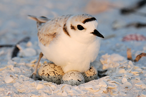
The data were collected at the Point Reyes National Seashore by a former student at Berkeley. The goal was to see how the size of an egg could be used to predict the weight of the resulting chick. The bigger the newly-hatched chick, the more likely it is to survive.

Each row of the data frame below corresponds to one Snowy Plover egg and the resulting chick. Note how tiny the bird is:
- Egg Length and Egg Breadth (widest diameter) are measured in millimeters
- Egg Weight and Bird Weight are measured in grams; for comparison, a standard paper clip weighs about one gram
eggs = pd.read_csv('data/snowy_plover.csv.gz')
eggs.head()
| egg_weight | egg_length | egg_breadth | bird_weight | |
|---|---|---|---|---|
| 0 | 7.4 | 28.80 | 21.84 | 5.2 |
| 1 | 7.7 | 29.04 | 22.45 | 5.4 |
| 2 | 7.9 | 29.36 | 22.48 | 5.6 |
| 3 | 7.5 | 30.10 | 21.71 | 5.3 |
| 4 | 8.3 | 30.17 | 22.75 | 5.9 |
eggs.shape
(44, 4)
For a particular egg, $x$ is the vector of length, breadth, and weight. The proposed model is
$$ \widehat{\text{Newborn weight}} = \hat{\theta}_0 + \hat{\theta}_1 \text{egg\_weight} + \hat{\theta}_2 \text{egg\_length} + \hat{\theta}_2 \text{egg\_breadth} $$
Let's fit this model:
y = eggs["bird_weight"]
X = eggs[["egg_weight", "egg_length", "egg_breadth"]]
model = lm.LinearRegression(fit_intercept=True).fit(X, y)
display(pd.DataFrame(
[model.intercept_] + list(model.coef_),
columns=['theta_hat'],
index=['intercept', 'egg_weight', 'egg_length', 'egg_breadth']))
all_features_rmse = np.mean((y - model.predict(X)) ** 2)
print("RMSE", all_features_rmse)
| theta_hat | |
|---|---|
| intercept | -4.605670 |
| egg_weight | 0.431229 |
| egg_length | 0.066570 |
| egg_breadth | 0.215914 |
RMSE 0.045470853802757616
Let's try bootstrapping the sample to obtain a 95% confidence intervals for all the parameters.
# This function returns a list of the coefficients of the fitted model
def all_thetas(sample):
model = lm.LinearRegression().fit(
sample[["egg_weight", "egg_length", "egg_breadth"]],
sample["bird_weight"])
return [model.intercept_] + model.coef_.tolist()
We can re-use our bootstrapping function from before to get synthetic estimates of all of the coefficients:
bs_thetas = pd.DataFrame(
bootstrap(eggs, all_thetas, 1000),
columns=['intercept', 'egg_weight', 'egg_length', 'egg_breadth'])
bs_thetas
Bootstrapping: 0%| | 0/1000 [00:00<?, ?it/s]
| intercept | egg_weight | egg_length | egg_breadth | |
|---|---|---|---|---|
| 0 | -8.103400 | 0.216451 | 0.098032 | 0.405838 |
| 1 | -11.074321 | 0.077284 | 0.148533 | 0.521490 |
| 2 | -2.718266 | 0.608443 | 0.035361 | 0.111554 |
| 3 | -1.080113 | 0.597081 | 0.026363 | 0.053714 |
| 4 | -2.124909 | 0.663734 | 0.002459 | 0.107473 |
| ... | ... | ... | ... | ... |
| 995 | 0.034319 | 0.965715 | -0.062090 | -0.009347 |
| 996 | -6.894141 | 0.288500 | 0.066708 | 0.368040 |
| 997 | -0.395814 | 0.695542 | -0.032516 | 0.068442 |
| 998 | -7.291577 | 0.499068 | 0.040360 | 0.344834 |
| 999 | -4.958756 | 0.428270 | 0.047167 | 0.258591 |
1000 rows × 4 columns
Computing the confidence intervals using the 1,000 synthetic estimates:
cis = (bs_thetas
.apply(bootstrap_ci).T
.rename(columns={0: 'lower', 1: 'upper'}))
cis
| lower | upper | |
|---|---|---|
| intercept | -14.740386 | 4.844829 |
| egg_weight | -0.219311 | 1.082662 |
| egg_length | -0.092170 | 0.208965 |
| egg_breadth | -0.230592 | 0.725745 |
def visualize_coeffs(bs_thetas, rows, cols):
cis = (bs_thetas
.apply(bootstrap_ci).T
.rename(columns={0: 'lower', 1: 'upper'}))
display(cis)
from plotly.subplots import make_subplots
fig = make_subplots(rows=rows, cols=cols, subplot_titles=cis.index)
for i, coeff_name in enumerate(cis.index):
c = (i % cols) + 1
r = (i // cols) + 1
fig.add_histogram(x=bs_thetas[coeff_name], name=coeff_name,
row=r, col=c, histnorm='probability')
fig.add_vline(x=0, row=r, col=c)
fig.add_vline(x=cis.loc[coeff_name, 'lower'], line=ci_line_style,
row=r, col=c)
fig.add_vline(x=cis.loc[coeff_name, 'upper'], line=ci_line_style,
row=r, col=c)
return fig
visualize_coeffs(bs_thetas, 2, 2)
| lower | upper | |
|---|---|---|
| intercept | -14.740386 | 4.844829 |
| egg_weight | -0.219311 | 1.082662 |
| egg_length | -0.092170 | 0.208965 |
| egg_breadth | -0.230592 | 0.725745 |
Because all the confidence intervals contain 0, we cannot reject the null hypothesis that the true coefficient on each term is 0.
Does this mean that all the parameters are statistically indistinguishable from 0?
Inspecting the Relationship between Features
To see what's going on, we'll make a scatter plot matrix for the data.
px.scatter_matrix(eggs, width=600, height=600)
This shows that bird_weight
is highly correlated with all the other
variables (the bottom row), which means fitting a linear model is a good idea.
But, we also see that egg_weight is highly correlated with all the variables
(the top row).
We saw in lecture that this could result in high variance coefficients and harm inference.
Here are the numeric correlations:
px.imshow(eggs.corr().round(2), text_auto=True, width=600)
Changing Our Modeling Features
Based on the correlations above, egg_weight looks like the strongest predictor of newborn chick weight.
An SLR model with just egg_weight performs almost as well as the model that uses all three variables, and the confidence interval for $\hat{\theta}_1$ no longer
contains zero.
- Note that the model with additional variables has a slightly lower RMSE! In sample RMSE will never go up when you add features.
y = eggs["bird_weight"]
X = eggs[["egg_weight"]]
model = lm.LinearRegression(fit_intercept=True).fit(X, y)
display(pd.DataFrame([model.intercept_] + list(model.coef_),
columns=['theta_hat'],
index=['intercept', 'egg_weight']))
print("All Features RMSE: ", all_features_rmse)
print("Simpler model RMSE: ", np.mean((y - model.predict(X)) ** 2))
| theta_hat | |
|---|---|
| intercept | -0.058272 |
| egg_weight | 0.718515 |
All Features RMSE: 0.045470853802757616 Simpler model RMSE: 0.046493941375556846
# Return a list of the intercept and slope of the SLR model using just egg_weight
def egg_weight_coeff(sample):
model = lm.LinearRegression().fit(
sample[["egg_weight"]],
sample["bird_weight"])
return [model.intercept_] + model.coef_.tolist()
We can re-use our bootstrap function from earlier to generate synthetic estimates of the coefficient on egg_weight:
bs_thetas_egg_weight = pd.DataFrame(
bootstrap(eggs, egg_weight_coeff, 1000),
columns=['intercept', 'egg_weight'])
bs_thetas_egg_weight
Bootstrapping: 0%| | 0/1000 [00:00<?, ?it/s]
| intercept | egg_weight | |
|---|---|---|
| 0 | -0.108481 | 0.721276 |
| 1 | 0.178621 | 0.687295 |
| 2 | 0.131337 | 0.698104 |
| 3 | -0.022869 | 0.712006 |
| 4 | 0.329215 | 0.669357 |
| ... | ... | ... |
| 995 | -0.776623 | 0.803877 |
| 996 | 0.130192 | 0.692799 |
| 997 | -0.540054 | 0.782740 |
| 998 | -0.498966 | 0.767973 |
| 999 | -0.221662 | 0.735186 |
1000 rows × 2 columns
visualize_coeffs(bs_thetas_egg_weight, 1, 2)
| lower | upper | |
|---|---|---|
| intercept | -0.783541 | 0.917632 |
| egg_weight | 0.602692 | 0.809269 |
Notice how much tighter the confidence interval is for egg_weight above, relative to the regression where we included all three collinear terms!
As this example shows, checking for collinearity is important for inference (and less so for prediction).
When we fit a model on highly correlated variables, confidence intervals can have high variance, preventing us from making meaningful statistical conclusions about the relationships between features and outputs.