Diversity and Data Science:
Unfortunately, surveys of data scientists suggest that there are far fewer women in data science:
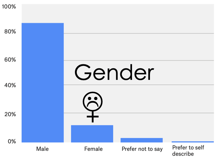
To learn more check out the Kaggle Executive Summary or study the Raw Data.
by Lisa Yan
adapted from Joseph E. Gonzalez, Anthony D. Joseph, Josh Hug, Suraj Rampure
The website links may often link to the JupyterLab view, where you can browse files and access the Terminal. You can click to hide the sidebar.
To view this notebook in Simple Notebook view (which helps conserve browser memory):
View -> Open With Classic Notebook, orlab from the URL.We will be using a wide range of different Python software packages. To install and manage these packages we will be using the Conda environment manager. The following is a list of packages we will routinely use in lectures and homeworks:
# linear algebra, probability
import numpy as np

# data manipulation
import pandas as pd

# visualization
import matplotlib.pyplot as plt
import seaborn as sns
%matplotlib inline

## interactive visualization library
import plotly.offline as py
py.init_notebook_mode()
import plotly.graph_objs as go
import plotly.figure_factory as ff
import plotly.express as px
We will learn how to use all of the technologies used in this demo.
For now, just sit back and think critically about the data and our guided analysis.
This is a pretty vague question but let's start with the goal of learning something about the students in the class.
Here are some "simple" questions:
In DS100 we will study various methods to collect data.
To answer this question, I downloaded the course roster and extracted everyone's names and majors.
# pd stands for pandas, which we will learn next week
# some pandas syntax shared with data8's datascience package
majors = pd.read_csv("data/majors.csv")
names = pd.read_csv("data/names.csv")
In DS100 we will study exploratory data analysis and practice analyzing new datasets.
I didn't tell you the details of the data! Let's check out the data and infer its structure. Then we can start answering the simple questions we posed.
majors.head(20)
| Majors | Terms in Attendance | |
|---|---|---|
| 0 | Letters & Sci Undeclared UG | 6 |
| 1 | Civil Engineering BS | 6 |
| 2 | Conserv & Resource Stds BS | 4 |
| 3 | Public Health MPH | G |
| 4 | Letters & Sci Undeclared UG | 2 |
| 5 | Data Science BA | 6 |
| 6 | Letters & Sci Undeclared UG | 4 |
| 7 | Cognitive Science BA, Computer Science BA | 6 |
| 8 | Environ Econ & Policy BS | 6 |
| 9 | Statistics BA | 7 |
| 10 | Letters & Sci Undeclared UG | 6 |
| 11 | Letters & Sci Undeclared UG | 4 |
| 12 | Letters & Sci Undeclared UG | 4 |
| 13 | Economics BA | 6 |
| 14 | Industrial Eng & Ops Rsch MEng | G |
| 15 | Computer Science BA | 6 |
| 16 | Civil & Env Eng Prof MS | G |
| 17 | Computer Science BA | 8 |
| 18 | Letters & Sci Undeclared UG | 6 |
| 19 | Cognitive Science BA | 8 |
names.head()
| Name | Role | |
|---|---|---|
| 0 | Kelly | Student |
| 1 | Joshua | Student |
| 2 | Peter | Student |
| 3 | HANNAH | Student |
| 4 | Ryan | Student |
Answer: Some names appear capitalized.
In the above sample we notice that some of the names are capitalized and some are not. This will be an issue in our later analysis so let's convert all names to lower case.
names['Name'] = names['Name'].str.lower()
names.head()
| Name | Role | |
|---|---|---|
| 0 | kelly | Student |
| 1 | joshua | Student |
| 2 | peter | Student |
| 3 | hannah | Student |
| 4 | ryan | Student |
print(len(names))
print(len(majors))
1125
1125
Based on what we know of our class, each record is most likely a student.
Q: Is this big data (would you call this a "big class")?
This would not normally constitute big data ... however this is a common data size for a lot of data analysis tasks.
Is this a big class? YES!
It is important that we understand the meaning of each field and how the data is organized.
names.head()
| Name | Role | |
|---|---|---|
| 0 | kelly | Student |
| 1 | joshua | Student |
| 2 | peter | Student |
| 3 | hannah | Student |
| 4 | ryan | Student |
Q: What is the meaning of the Role field?
A: Understanding the meaning of field can often be achieved by looking at the types of data it contains (in particular the counts of its unique values).
We use the value_counts() function in pandas:
names['Role'].value_counts().to_frame() # counts of unique Roles
| Role | |
|---|---|
| Student | 1100 |
| Waitlist Student | 24 |
| #REF! | 1 |
It appears that one student has an erroneous role given as "#REF!". What else can we learn about this student? Let's see their name.
# boolean index to find rows where Role is #REF!
names[names['Role'] == "#REF!"]
| Name | Role | |
|---|---|---|
| 146 | #ref! | #REF! |
Though this single bad record won't have much of an impact on our analysis, we can clean our data by removing this record.
names = names[names['Role'] != "#REF!"]
Double check: Let's double check that our record removal only removed the single bad record.
names['Role'].value_counts().to_frame() # again, counts of unique Roles
| Role | |
|---|---|
| Student | 1100 |
| Waitlist Student | 24 |
Remember we loaded in two files. Let's explore the fields of majors and check for bad records:
majors.columns # get column names
Index(['Majors', 'Terms in Attendance'], dtype='object')
majors['Terms in Attendance'].value_counts().to_frame()
| Terms in Attendance | |
|---|---|
| 4 | 362 |
| 6 | 311 |
| G | 199 |
| 8 | 140 |
| 7 | 39 |
| 2 | 35 |
| 5 | 31 |
| 3 | 4 |
| U | 3 |
| #REF! | 1 |
It looks like numbers represents semesters, G represents graduate students, and U might represent something else---maybe campus visitors. But we do still have a bad record:
majors[majors['Terms in Attendance'] == "#REF!"]
| Majors | Terms in Attendance | |
|---|---|---|
| 683 | #REF! | #REF! |
majors = majors[majors['Terms in Attendance'] != "#REF!"]
majors['Terms in Attendance'].value_counts().to_frame()
| Terms in Attendance | |
|---|---|
| 4 | 362 |
| 6 | 311 |
| G | 199 |
| 8 | 140 |
| 7 | 39 |
| 2 | 35 |
| 5 | 31 |
| 3 | 4 |
| U | 3 |
Detail: The deleted majors record number 683 is different from the record number (146) of the bad names record. So while the number of records in each table matches, the row indices don't match, so we'll have to keep these tables separate in order to do our analysis.
We will often want to numerically or visually summarize the data. The describe() method provides a brief high level description of our data frame.
names.describe()
| Name | Role | |
|---|---|---|
| count | 1124 | 1124 |
| unique | 881 | 2 |
| top | ryan | Student |
| freq | 9 | 1100 |
majors.describe()
| Majors | Terms in Attendance | |
|---|---|---|
| count | 1124 | 1124 |
| unique | 147 | 9 |
| top | Letters & Sci Undeclared UG | 4 |
| freq | 357 | 362 |
Q: What do you think top and freq represent?
A: top: most frequent entry, freq: the frequency of that entry
What are the top majors:
majors_count = (       # method chaining in pandas
    majors['Majors']
    .value_counts()
    .sort_values(ascending=True) # lowest first
    .to_frame()
    .tail(20)          # get the top 20
)

# or, comment out to parse double majors
# majors_count = (
#     majors['Majors']
#     .str.split(", ") # get double majors
#     .explode()       # one major to every row
#     .value_counts()
#     .sort_values(ascending=True)
#     .to_frame()
#     .tail(20)
# )

majors_count
| Majors | |
|---|---|
| Bioengineering BS | 6 |
| Statistics BA | 6 |
| Civil & Environmental Eng MEng | 7 |
| Info Mgmt & Systems MIMS | 8 |
| Molecular & Cell Biology BA | 8 |
| Public Health BA | 9 |
| Business Administration BS | 10 |
| Civil & Env Eng Prof MS | 13 |
| Chemical Engineering BS | 13 |
| Applied Mathematics BA | 14 |
| Public Health MPH | 17 |
| Industrial Eng & Ops Rsch MEng | 32 |
| Cognitive Science BA | 33 |
| Electrical Eng & Comp Sci BS | 39 |
| Electrical Eng & Comp Sci MEng | 42 |
| Economics BA | 46 |
| Civil Engineering BS | 55 |
| Data Science BA | 66 |
| Computer Science BA | 96 |
| Letters & Sci Undeclared UG | 357 |
In DS100 we will deal with many different kinds of data (not just numbers) and we will study techniques to diverse types of data.
How can we summarize the Majors field? A good starting point might be to use a bar plot:
# interactive using plotly
fig = px.bar(majors_count, orientation='h')
fig.update_layout(showlegend=False,
                  xaxis_title='Count',
                  yaxis_title='Major')
fig = px.histogram(majors['Terms in Attendance'].sort_values(),
                   histnorm='probability')
fig.update_layout(showlegend=False,
                  xaxis_title="Term",
                  yaxis_title="Fraction of Class")
Unfortunately, surveys of data scientists suggest that there are far fewer women in data science:
To learn more check out the Kaggle Executive Summary or study the Raw Data.
I actually get asked this question a lot as we try to improve the data science program at Berkeley.
This is actually a fairly complex question. What do we mean by female? Is this a question about the sex or gender identity of the students? They are not the same thing.
Most likely, my colleagues are interested in improving gender diversity, by ensuring that our program is inclusive. Let's reword this question:
print(majors.columns)
print(names.columns)
Index(['Majors', 'Terms in Attendance'], dtype='object')
Index(['Name', 'Role'], dtype='object')
Please do not attempt option (2) alone. What I am about to do is flawed in so many ways and we will discuss these flaws in a moment and throughout the semester.
However, it will illustrate some very basic inferential modeling and how we might combine multiple data sources to try and reason about something we haven't measured.
To attempt option (2), we will first look at a second data source.
To study what a name tells about a person we will download data from the United States Social Security office containing the number of registered names broken down by year, sex, and name. This is often called the Baby Names Data as social security numbers (SSNs) are typically given at birth.
A: In this demo we'll use a person's name to estimate their sex. But a person's name tells us many things (more on this later).
Note 1: In the following we download the data programmatically to ensure that the process is reproducible.
Note 2: We also load the data directly into python without decompressing the zipfile.
In DS100 we will think a bit more about how we can be efficient in our data analysis to support processing large datasets.
import urllib.request
import os.path

# Download data from the web directly
data_url = "https://www.ssa.gov/oact/babynames/names.zip"
local_filename = "babynames.zip"
if not os.path.exists(local_filename): # if the data exists don't download again
    with urllib.request.urlopen(data_url) as resp, open(local_filename, 'wb') as f:
        f.write(resp.read())


# Load data without unzipping the file
import zipfile
babynames = []
with zipfile.ZipFile(local_filename, "r") as zf:
    data_files = [f for f in zf.filelist if f.filename[-3:] == "txt"]
    def extract_year_from_filename(fn):
        return int(fn[3:7])
    for f in data_files:
        year = extract_year_from_filename(f.filename)
        with zf.open(f) as fp:
            df = pd.read_csv(fp, names=["Name", "Sex", "Count"])
            df["Year"] = year
            babynames.append(df)
babynames = pd.concat(babynames)


babynames.head() # show the first few rows
| Name | Sex | Count | Year | |
|---|---|---|---|---|
| 0 | Mary | F | 7065 | 1880 |
| 1 | Anna | F | 2604 | 1880 |
| 2 | Emma | F | 2003 | 1880 |
| 3 | Elizabeth | F | 1939 | 1880 |
| 4 | Minnie | F | 1746 | 1880 |
In Data 100 you will have to learn about different data sources (and their limitations) on your own.
Reading from SSN Office description, bolded for readability:
All names are from Social Security card applications for births that occurred in the United States after 1879. Note that many people born before 1937 never applied for a Social Security card, so their names are not included in our data. For others who did apply, our records may not show the place of birth, and again their names are not included in our data.
To safeguard privacy, we exclude from our tabulated lists of names those that would indicate, or would allow the ability to determine, names with fewer than 5 occurrences in any geographic area. If a name has less than 5 occurrences for a year of birth in any state, the sum of the state counts for that year will be less than the national count.
All data are from a 100% sample of our records on Social Security card applications as of March 2021.
Examining the data:
babynames
| Name | Sex | Count | Year | |
|---|---|---|---|---|
| 0 | Mary | F | 7065 | 1880 |
| 1 | Anna | F | 2604 | 1880 |
| 2 | Emma | F | 2003 | 1880 |
| 3 | Elizabeth | F | 1939 | 1880 |
| 4 | Minnie | F | 1746 | 1880 |
| ... | ... | ... | ... | ... |
| 31266 | Zykell | M | 5 | 2020 |
| 31267 | Zylus | M | 5 | 2020 |
| 31268 | Zymari | M | 5 | 2020 |
| 31269 | Zyn | M | 5 | 2020 |
| 31270 | Zyran | M | 5 | 2020 |
2020863 rows × 4 columns
In our earlier analysis we converted names to lower case. We will do the same again here:
babynames['Name'] = babynames['Name'].str.lower()
babynames.head()
| Name | Sex | Count | Year | |
|---|---|---|---|---|
| 0 | mary | F | 7065 | 1880 |
| 1 | anna | F | 2604 | 1880 |
| 2 | emma | F | 2003 | 1880 |
| 3 | elizabeth | F | 1939 | 1880 |
| 4 | minnie | F | 1746 | 1880 |
How many people does this data represent?
format(babynames['Count'].sum(), ',d') # sum of 'Count' column
'358,480,709'
format(len(babynames), ',d') # number of rows
'2,020,863'
Q: Is this number low or high?
Answer
It seems low (the 2020 US population was 329.5 million). However the social security website states:
All names are from Social Security card applications for births that occurred in the United States after 1879. Note that many people born before 1937 never applied for a Social Security card, so their names are not included in our data. For others who did apply, our records may not show the place of birth, and again their names are not included in our data. All data are from a 100% sample of our records on Social Security card applications as of the end of February 2016.
Trying a simple query using query:
# how many Nora's were born in 2018?
babynames[(babynames['Name'] == 'nora') & (babynames['Year'] == 2018)]
| Name | Sex | Count | Year | |
|---|---|---|---|---|
| 29 | nora | F | 5833 | 2018 |
| 28514 | nora | M | 7 | 2018 |
Trying a more complex query using query() (to be discussed next week):
# how many baby names contain the word "data"?
babynames.query('Name.str.contains("data")', engine='python')
| Name | Sex | Count | Year | |
|---|---|---|---|---|
| 9764 | kidata | F | 5 | 1975 |
| 24915 | datavion | M | 5 | 1995 |
| 23610 | datavious | M | 7 | 1997 |
| 12103 | datavia | F | 7 | 2000 |
| 27508 | datavion | M | 6 | 2001 |
| 28913 | datari | M | 5 | 2001 |
| 29140 | datavian | M | 5 | 2002 |
| 29141 | datavious | M | 5 | 2002 |
| 30573 | datavion | M | 5 | 2004 |
| 17139 | datavia | F | 5 | 2005 |
| 31030 | datavion | M | 5 | 2005 |
| 31023 | datavion | M | 6 | 2006 |
| 33341 | datavious | M | 5 | 2007 |
| 33342 | datavius | M | 5 | 2007 |
| 33403 | datavious | M | 5 | 2008 |
| 33081 | datavion | M | 5 | 2009 |
| 32497 | datavious | M | 5 | 2010 |
In DS100 we still study how to visualize and analyze relationships in data.
In this example we construct a pivot table which aggregates the number of babies registered for each year by Sex.
We'll discuss pivot tables in detail next week.
# counts number of M and F babies per year
year_sex = pd.pivot_table(
        babynames,
        index=['Year'], # the row index
        columns=['Sex'], # the column values
        values='Count', # the field(s) to processed in each group
        aggfunc=np.sum,
    )[["M", "F"]]

year_sex.head()
| Sex | M | F |
|---|---|---|
| Year | ||
| 1880 | 110490 | 90994 |
| 1881 | 100738 | 91953 |
| 1882 | 113686 | 107847 |
| 1883 | 104625 | 112319 |
| 1884 | 114442 | 129019 |
We can visualize these descriptive statistics:
# more interactive using plotly
fig = px.line(year_sex)
fig.update_layout(title="Total Babies per Year",
                  yaxis_title="Number of Babies")
# counts number of M and F *names* per year
year_sex_unique = pd.pivot_table(babynames,
        index=['Year'],
        columns=['Sex'],
        values='Name',
        aggfunc=lambda x: len(np.unique(x)),
    )
fig = px.line(year_sex_unique)
fig.update_layout(title="Unique Names Per Year",
                  yaxis_title="Number of Baby Names")
Some observations:
Let's use the Baby Names dataset to estimate the fraction of female students in the class.
First, we construct a pivot table to compute the total number of babies registered for each Name, broken down by Sex.
# counts number of M and F babies per name
name_sex = pd.pivot_table(babynames, index='Name', columns='Sex', values='Count',
                            aggfunc='sum', fill_value=0., margins=True)
name_sex.head()
| Sex | F | M | All |
|---|---|---|---|
| Name | |||
| aaban | 0 | 120 | 120 |
| aabha | 46 | 0 | 46 |
| aabid | 0 | 16 | 16 |
| aabidah | 5 | 0 | 5 |
| aabir | 0 | 10 | 10 |
Second, we compute proportion of female babies for each name. This is our estimated probability that the baby is Female:
$$ \hat{\textbf{P}\hspace{0pt}}(\text{Female} \,\,\, | \,\,\, \text{Name} ) = \frac{\textbf{Count}(\text{Female and Name})}{\textbf{Count}(\text{Name})} $$prop_female = (name_sex['F'] / name_sex['All']).rename("Prop. Female")
prop_female.to_frame().head(10)
| Prop. Female | |
|---|---|
| Name | |
| aaban | 0.0 |
| aabha | 1.0 |
| aabid | 0.0 |
| aabidah | 1.0 |
| aabir | 0.0 |
| aabriella | 1.0 |
| aada | 1.0 |
| aadam | 0.0 |
| aadan | 0.0 |
| aadarsh | 0.0 |
prop_female["lisa"]
0.9971226839257452
prop_female["josh"]
0.0
prop_female["avery"]
0.7021478300997172
prop_female["min"]
0.37598736176935227
prop_female["pat"]
0.6001495774437214
prop_female["jaspreet"]
0.6043956043956044
We can define a function to return the most likely Sex for a name. If there is an exact tie or the name does not appear in the social security dataset the function returns Unknown.
def sex_from_name(name):
    lower_name = name.lower()
    if lower_name not in prop_female.index or prop_female[lower_name] == 0.5:
        return "Unknown"
    elif prop_female[lower_name] > 0.5:
        return "F"
    else:
        return "M"
sex_from_name("nora")
'F'
sex_from_name("josh")
'M'
sex_from_name("pat")
'F'
Let's try out our simple classifier! We'll use the apply() function to classify each student name:
# apply sex_from_name to each student name
names['Pred. Sex'] = names['Name'].apply(sex_from_name)
px.bar(names['Pred. Sex'].value_counts()/len(names))
That's a lot of Unknowns.
...But we can still estimate the fraction of female students in the class:
count_by_sex = names['Pred. Sex'].value_counts().to_frame()
count_by_sex
| Pred. Sex | |
|---|---|
| M | 523 |
| F | 394 |
| Unknown | 207 |
count_by_sex.loc['F']/(count_by_sex.loc['M'] + count_by_sex.loc['F'])
Pred. Sex    0.429662
dtype: float64
Questions:
Q: What fraction of students in Data 100 this semester have names in the SSN dataset?
print("Fraction of names in the babynames data:",
      names['Name'].isin(prop_female.index).mean())
Fraction of names in the babynames data: 0.8158362989323843
Q: Which names are not in the dataset?
Why might these names not appear?
# the tilde ~ negates the boolean index. More next week.
names[~names['Name'].isin(prop_female.index)].sample(10)
| Name | Role | Pred. Sex | |
|---|---|---|---|
| 185 | linchuan | Student | Unknown |
| 541 | milgo | Student | Unknown |
| 245 | trishala | Student | Unknown |
| 774 | mengmeng | Student | Unknown |
| 1114 | bukun | Student | Unknown |
| 337 | jiaping | Student | Unknown |
| 414 | ajitika | Student | Unknown |
| 909 | caedi | Student | Unknown |
| 590 | anjika | Student | Unknown |
| 209 | cat | Student | Unknown |
Previously we treated a name which is given to females 40% of the time as a "Male" name, because the probability was less than 0.5. This doesn't capture our uncertainty.
We can use simulation to provide a better distributional estimate. We'll use 50% for names not in the Baby Names dataset.
# add the computed SSN F proportion to each row. 0.5 for Unknowns.
# merge() effectively "join"s two tables together. to be covered next week.
names['Prop. Female'] = (
    names[['Name']].merge(prop_female, how='left', left_on='Name',
                          right_index=True)['Prop. Female']
        .fillna(0.5)
)
names.head(10)
| Name | Role | Pred. Sex | Prop. Female | |
|---|---|---|---|---|
| 0 | kelly | Student | F | 0.852264 |
| 1 | joshua | Student | M | 0.004019 |
| 2 | peter | Student | M | 0.003328 |
| 3 | hannah | Student | F | 0.998415 |
| 4 | ryan | Student | M | 0.026049 |
| 5 | ryan | Student | M | 0.026049 |
| 6 | kevin | Student | M | 0.004517 |
| 7 | justin | Student | M | 0.004840 |
| 8 | alex | Student | M | 0.032375 |
| 9 | jessica | Student | F | 0.996598 |
# if a randomly picked number from [0.0, 1.0) is under the Female proportion, then F
names['Sim. Female'] = np.random.rand(len(names)) < names['Prop. Female']
names.tail(20)
| Name | Role | Pred. Sex | Prop. Female | Sim. Female | |
|---|---|---|---|---|---|
| 1105 | sofiya | Student | F | 1.000000 | True |
| 1106 | heming | Student | Unknown | 0.500000 | True |
| 1107 | armaan | Student | M | 0.000000 | False |
| 1108 | paul | Student | M | 0.004182 | False |
| 1109 | hans | Student | M | 0.000334 | False |
| 1110 | lois | Student | F | 0.992124 | True |
| 1111 | richard | Student | M | 0.003696 | False |
| 1112 | mehdi | Waitlist Student | M | 0.000000 | False |
| 1113 | kyle | Student | M | 0.017914 | False |
| 1114 | bukun | Student | Unknown | 0.500000 | True |
| 1115 | ansh | Student | M | 0.000000 | False |
| 1116 | nick | Student | M | 0.002645 | False |
| 1117 | haohan | Student | Unknown | 0.500000 | True |
| 1118 | bretton | Student | M | 0.000000 | False |
| 1119 | samhith | Student | M | 0.000000 | False |
| 1120 | megan | Student | F | 0.997486 | True |
| 1121 | nikitha | Student | F | 1.000000 | True |
| 1122 | jinsong | Student | Unknown | 0.500000 | True |
| 1123 | tobias | Student | M | 0.000000 | False |
| 1124 | selina | Student | F | 1.000000 | True |
Given such a simulation, we can compute the fraction of the class that is female.
# proportion of Trues in the 'Sim. Female' column
names['Sim. Female'].mean()
0.45640569395017794
Now that we're performing a simulation, the above proportion is random: it depends on the random numbers we picked to determine whether a student was Female.
Let's run the above simulation several times and see what the distribution of this Female proportion is. The below cell may take a few seconds to run.
# function that performs many simulations
def simulate_class(students):
    is_female = names['Prop. Female'] > np.random.rand(len(names['Prop. Female']))
    return np.mean(is_female)

sim_frac_female = np.array([simulate_class(names) for n in range(10000)])
fig = ff.create_distplot([sim_frac_female], ['Fraction Female'], bin_size=0.0025, show_rug=False)
fig.update_layout(xaxis_title='Prop. Female',
                  yaxis_title='Percentage',
                  title='Distribution of Simulated Proportions of Females in the Class')
ax = sns.histplot(sim_frac_female, stat='probability', kde=True, bins=20)
sns.rugplot(sim_frac_female, ax=ax)
ax.set_xlabel("Fraction Female")
ax.set_title('Distribution of Simulated Fractions Female in the Class');

In DS100 we will understand Kernel Density Functions, Rug Plots, and other visualization techniques.
We saw with our Simple Classifier that many student names were classified as "Unknown," often because they weren't in the SSN Baby Names Dataset.
Recall the SSN dataset:
All names are from Social Security card applications for births that occurred in the United States after 1879.
That statement is not reflective of all of our students!!
# students who were not in the SSN Baby Names Dataset
names[~names['Name'].isin(prop_female.index)].sample(10)
| Name | Role | Pred. Sex | Prop. Female | Sim. Female | |
|---|---|---|---|---|---|
| 553 | raag | Student | Unknown | 0.5 | False |
| 18 | xingrong | Student | Unknown | 0.5 | True |
| 985 | sehee | Student | Unknown | 0.5 | True |
| 988 | gurkaran | Student | Unknown | 0.5 | True |
| 298 | ningyu | Student | Unknown | 0.5 | True |
| 712 | rabail | Student | Unknown | 0.5 | True |
| 774 | mengmeng | Student | Unknown | 0.5 | True |
| 91 | prasuna | Student | Unknown | 0.5 | True |
| 1011 | shomini | Student | Unknown | 0.5 | True |
| 185 | linchuan | Student | Unknown | 0.5 | False |
Using data from 1879 (or even 1937) does not represent the diversity and context of U.S. baby names today.
Here are some choice names to show you how the distribution of particular names has varied with time:
subset_names = ["edris", "jamie", "jordan", "leslie", "taylor", "willie"]
subset_babynames_year = (pd.pivot_table(
                    babynames[babynames['Name'].isin(subset_names)],
                    index=['Name', 'Year'], columns='Sex', values='Count',
                    aggfunc='sum', fill_value=0, margins=True)
                 .drop(labels='All', level=0, axis=0) # drop cumulative row
                 .rename_axis(None, axis=1) # remove pivot table col name
                 .reset_index() # move (name, year) back into columns
                 .assign(Propf = lambda row: row.F/(row.F + row.M))
                )
ax = sns.lineplot(data=subset_babynames_year,
                  x='Year', y='Propf', hue='Name')
ax.set_title("Ratio of Female Babies over Time for Select Names")
ax.set_ylabel("Proportion of Female Names in a Year")
ax.legend(loc="lower left");

Curious as to how we got the above names? We picked out two types of names:
Check it out:
"""
get a subset of names that:
    have had propf above a threshold, as well as
    have been counted for more than a certain number of years
Note: while we could do our analysis over all names,
    it turns out many names don't matter.
    So to save computation power, we just work
    with a subset of names we know may be candidates.
"""
# these are thresholds we set as data analysts
propf_min = 0.2
propf_max = 0.8
year_thresh = 30

propf_countyear = (babynames
                   .groupby('Name').count()
                   .merge(prop_female.to_frame(), on='Name')
                   .rename(columns={'Prop. Female': 'Propf'})
                   .query("@propf_min < Propf < @propf_max & Year > @year_thresh & Name != 'All'")
                  )[['Propf', 'Year']]
propf_countyear
| Propf | Year | |
|---|---|---|
| Name | ||
| aalijah | 0.379135 | 38 |
| aamari | 0.396694 | 32 |
| aaren | 0.246719 | 72 |
| aarin | 0.296369 | 74 |
| aarion | 0.227061 | 57 |
| ... | ... | ... |
| zephyr | 0.242366 | 72 |
| ziah | 0.753100 | 41 |
| zian | 0.204607 | 42 |
| ziyan | 0.445946 | 33 |
| zyan | 0.212121 | 48 |
1572 rows × 2 columns
# construct a pivot table of (name, year) to count
keep_names = propf_countyear.reset_index()['Name']
name_year_sex = (pd.pivot_table(
                    babynames[babynames['Name'].isin(keep_names)],
                    index=['Name', 'Year'], columns='Sex', values='Count',
                    aggfunc='sum', fill_value=0, margins=True)
                 .drop(labels='All', level=0, axis=0) # drop cumulative row
                 .rename_axis(None, axis=1) # remove pivot table col name
                 .reset_index() # move (name, year) back into columns
                 .assign(Propf = lambda row: row.F/(row.F + row.M))
                )
name_year_sex
| Name | Year | F | M | All | Propf | |
|---|---|---|---|---|---|---|
| 0 | aalijah | 1994 | 5 | 0 | 5 | 1.000000 |
| 1 | aalijah | 1995 | 5 | 0 | 5 | 1.000000 |
| 2 | aalijah | 1999 | 5 | 0 | 5 | 1.000000 |
| 3 | aalijah | 2001 | 9 | 0 | 9 | 1.000000 |
| 4 | aalijah | 2002 | 9 | 6 | 15 | 0.600000 |
| ... | ... | ... | ... | ... | ... | ... |
| 85861 | zyan | 2016 | 15 | 74 | 89 | 0.168539 |
| 85862 | zyan | 2017 | 9 | 78 | 87 | 0.103448 |
| 85863 | zyan | 2018 | 6 | 88 | 94 | 0.063830 |
| 85864 | zyan | 2019 | 11 | 87 | 98 | 0.112245 |
| 85865 | zyan | 2020 | 6 | 84 | 90 | 0.066667 |
85866 rows × 6 columns
"""
Compute two statistics per name:
- Count of number of babies with name
- Variance of proportion of females
  (i.e., how much the proportion of females varied
  across different years)
"""
names_to_include = 40
group_names =  (name_year_sex
                       .groupby('Name')
                       .agg({'Propf': 'var', 'All': 'sum'})
                       .rename(columns={'Propf': 'Propf Var', 'All': 'Total'})
                       .reset_index()
                      )
# pick some high variance names
high_variance_names = (group_names
                       .sort_values('Propf Var', ascending=False)
                       .head(names_to_include)
                       .sort_values('Total', ascending=False)
                      )

high_variance_names.head(5)
| Name | Propf Var | Total | |
|---|---|---|---|
| 20 | aime | 0.240192 | 2235 |
| 932 | linzy | 0.226588 | 1498 |
| 950 | luan | 0.252718 | 1126 |
| 456 | edris | 0.225756 | 1013 |
| 931 | linzie | 0.246406 | 894 |
# pick some common names
common_names = (group_names
                .sort_values('Total', ascending=False)
                .head(names_to_include)
               )
common_names.head(10)
| Name | Propf Var | Total | |
|---|---|---|---|
| 1531 | willie | 0.026465 | 595556 |
| 707 | jordan | 0.012104 | 515701 |
| 1431 | taylor | 0.107966 | 435595 |
| 920 | leslie | 0.147283 | 380951 |
| 632 | jamie | 0.020379 | 355347 |
| 72 | angel | 0.032311 | 338457 |
| 907 | lee | 0.005258 | 293941 |
| 685 | jessie | 0.027374 | 278828 |
| 995 | marion | 0.017969 | 260844 |
| 349 | dana | 0.059260 | 245490 |