import numpy as np
import pandas as pd
import plotly.graph_objects as go
import plotly.express as px
import plotly.figure_factory as ff
from plotly.subplots import make_subplots
from sklearn.linear_model import LinearRegression
from sklearn.metrics import mean_squared_error
from sklearn.metrics import mean_absolute_error
In this notebook, we discuss:
In the process, we will work through feature engineering to construct a model that predicts vehicle efficiency.
For this notebook, we will use the seaborn mpg
data set which describes the fuel mileage (measured in miles per gallon or mpg) of various cars along with characteristics of those cars. Our goal will be to build a model that can predict the fuel mileage of a car based on the characteristics of that car.
from seaborn import load_dataset
data = load_dataset("mpg")
data
mpg | cylinders | displacement | horsepower | weight | acceleration | model_year | origin | name | |
---|---|---|---|---|---|---|---|---|---|
0 | 18.0 | 8 | 307.0 | 130.0 | 3504 | 12.0 | 70 | usa | chevrolet chevelle malibu |
1 | 15.0 | 8 | 350.0 | 165.0 | 3693 | 11.5 | 70 | usa | buick skylark 320 |
2 | 18.0 | 8 | 318.0 | 150.0 | 3436 | 11.0 | 70 | usa | plymouth satellite |
3 | 16.0 | 8 | 304.0 | 150.0 | 3433 | 12.0 | 70 | usa | amc rebel sst |
4 | 17.0 | 8 | 302.0 | 140.0 | 3449 | 10.5 | 70 | usa | ford torino |
... | ... | ... | ... | ... | ... | ... | ... | ... | ... |
393 | 27.0 | 4 | 140.0 | 86.0 | 2790 | 15.6 | 82 | usa | ford mustang gl |
394 | 44.0 | 4 | 97.0 | 52.0 | 2130 | 24.6 | 82 | europe | vw pickup |
395 | 32.0 | 4 | 135.0 | 84.0 | 2295 | 11.6 | 82 | usa | dodge rampage |
396 | 28.0 | 4 | 120.0 | 79.0 | 2625 | 18.6 | 82 | usa | ford ranger |
397 | 31.0 | 4 | 119.0 | 82.0 | 2720 | 19.4 | 82 | usa | chevy s-10 |
398 rows × 9 columns
This data set has several quantitative continuous features that we can use to build our first model. However, even for quantitative continuous features, we may want to do some additional feature engineering. Things to consider are:
We can use the Pandas DataFrame.isna
function to find rows with missing values:
data[data.isna().any(axis=1)]
mpg | cylinders | displacement | horsepower | weight | acceleration | model_year | origin | name | |
---|---|---|---|---|---|---|---|---|---|
32 | 25.0 | 4 | 98.0 | NaN | 2046 | 19.0 | 71 | usa | ford pinto |
126 | 21.0 | 6 | 200.0 | NaN | 2875 | 17.0 | 74 | usa | ford maverick |
330 | 40.9 | 4 | 85.0 | NaN | 1835 | 17.3 | 80 | europe | renault lecar deluxe |
336 | 23.6 | 4 | 140.0 | NaN | 2905 | 14.3 | 80 | usa | ford mustang cobra |
354 | 34.5 | 4 | 100.0 | NaN | 2320 | 15.8 | 81 | europe | renault 18i |
374 | 23.0 | 4 | 151.0 | NaN | 3035 | 20.5 | 82 | usa | amc concord dl |
There are many ways to deal with missing values. A common strategy is to substitute the mean. Because missing values can actually be useful signal, it is often a good idea to include a feature indicating that the value was missing.
def phi_cont(df):
Phi = df[["cylinders", "displacement",
"horsepower", "weight",
"acceleration",
"model_year"]].copy()
Phi["horsepower_missing"] = Phi["horsepower"].isna()
Phi = Phi.fillna(Phi.mean())
return Phi
Using our feature function, we can fit our first model to the transformed data:
model = LinearRegression()
model.fit(phi_cont(data), data[["mpg"]])
LinearRegression()
Because we are going to be building multiple models with different feature functions it is important to have a standard way to track each of the models.
The following function takes a model prediction function, the name of a model, and the dictionary of models that we have already constructed. It then evaluates the new model on the data and plots how the new model performs relative to the previous models as well as the $Y$ vs $\hat{Y}$ scatter plot.
In addition, it updates the dictionary of models to include the new model for future plotting.
def evaluate_model(name, model, phi, models=dict()):
# run the prediction function and compute the RMSE
Yhat = model.predict(phi(data)).flatten()
Y = data['mpg'].to_numpy()
rmse = np.sqrt(mean_squared_error(Y, Yhat))
print("Root Mean Squared Error:", rmse)
# Save the model and rmse to the collection of models
models[name] = dict(model=model, phi=phi, rmse=rmse)
# Generate diagnostic and model comparison plots
fig = make_subplots(rows=1, cols=2)
fig.add_trace(go.Scatter(x=Yhat, y=Y, mode="markers"), row=1, col=1)
fig.update_xaxes(title = "Yhat", row=1, col=1)
fig.update_yaxes(title = "Y", row=1, col=1)
ymin = np.min(Yhat)
ymax = np.max(Yhat)
fig.add_trace(go.Scatter(x=[ymin,ymax], y=[ymin,ymax], name="y=yhat"), row=1, col=1)
fig.add_trace(go.Bar(x=list(models.keys()),
y=[models[k]['rmse'] for k in models]), row=1, col=2)
fig.update_layout(showlegend=False)
fig.update_yaxes(title = "RMSE", row=1, col=2)
fig.show()
models = {}
evaluate_model("cont.", model, phi_cont, models)
Root Mean Squared Error: 3.4140204828031737
Unfortunately, the feature function we just implemented applies a different transformation depending on what input we provide. Specifically, if the horesepower
is missing when we go to make a prediction we will substitute it with a different mean then was used when we fit our model. Furthermore, if we only want predictions on a few records and the horsepower
is missing from those records then the feature function will be unable to substitute a meaningful value.
For example, if we were to get new records that look like the following:
new_data = data[data['horsepower'].isna()].head(3)
new_data
mpg | cylinders | displacement | horsepower | weight | acceleration | model_year | origin | name | |
---|---|---|---|---|---|---|---|---|---|
32 | 25.0 | 4 | 98.0 | NaN | 2046 | 19.0 | 71 | usa | ford pinto |
126 | 21.0 | 6 | 200.0 | NaN | 2875 | 17.0 | 74 | usa | ford maverick |
330 | 40.9 | 4 | 85.0 | NaN | 1835 | 17.3 | 80 | europe | renault lecar deluxe |
The feature function is be unable to substitute the mean since none of the records have a horsepower
value.
try:
model.predict(phi_cont(new_data))
except Exception as e:
print(e)
Input contains NaN, infinity or a value too large for dtype('float64').
We can fix this by computing the mean on the original data and using that mean on any new data.
# Making a global variable
def phi_cont(df, data_mean = data.mean()):
feature_cols = ["cylinders", "displacement", "horsepower", "weight", "acceleration", "model_year"]
Phi = df[feature_cols].copy()
Phi["horsepower_missing"] = Phi["horsepower"].isna().astype(float)
Phi = Phi.fillna(data_mean)
return Phi
model.predict(phi_cont(new_data))
array([[25.91611313], [22.40066016], [33.96492047]])
Because these kinds of transformations are fairly common. Scikit-learn has built-in transformations for data imputation. These transformations have a common pattern of fit
and transform
. You first fit
the transformation to your data and then you can transform
your data and any future data using the same transformation.
from sklearn.impute import SimpleImputer
imputer = SimpleImputer(strategy="mean")
imputer.fit(data[['weight', 'horsepower']])
SimpleImputer()
imputer.transform(data[['weight', 'horsepower']])[32]
array([2046. , 104.46938776])
imputer.fit(data[['horsepower']])
def phi_cont(df, imputer=imputer):
feature_cols = ["cylinders", "displacement", "horsepower", "weight", "acceleration", "model_year"]
Phi = df[feature_cols].copy()
Phi["horsepower_missing"] = Phi["horsepower"].isna().astype(float)
Phi["horsepower"] = imputer.transform(Phi[["horsepower"]]).flatten()
return Phi
model = LinearRegression()
model.fit(phi_cont(data), data[["mpg"]])
evaluate_model("cont.", model, phi_cont, models)
Root Mean Squared Error: 3.4140204828031737
The displacement of an engine is defined as the product of the volume of each cylinder and number of cylinders. However, not all cylinders fire at the same time (at least in a functioning engine) so the fuel economy might be more closely related to the volume of any one cylinder.
We can use this "domain knowledge" to compute a new feature encoding the volume per cylinder by taking the ratio of displacement and cylinders.
def phi_with_displacement(df):
Phi = phi_cont(df)
Phi['displacement/cylinder'] = Phi['displacement'] / Phi['cylinders']
return Phi
phi_with_displacement(data).head()
cylinders | displacement | horsepower | weight | acceleration | model_year | horsepower_missing | displacement/cylinder | |
---|---|---|---|---|---|---|---|---|
0 | 8 | 307.0 | 130.0 | 3504 | 12.0 | 70 | 0.0 | 38.375 |
1 | 8 | 350.0 | 165.0 | 3693 | 11.5 | 70 | 0.0 | 43.750 |
2 | 8 | 318.0 | 150.0 | 3436 | 11.0 | 70 | 0.0 | 39.750 |
3 | 8 | 304.0 | 150.0 | 3433 | 12.0 | 70 | 0.0 | 38.000 |
4 | 8 | 302.0 | 140.0 | 3449 | 10.5 | 70 | 0.0 | 37.750 |
Again fitting and evaluating our model we see a reduction in prediction error (RMSE).
model = LinearRegression()
model.fit(phi_with_displacement(data), data[["mpg"]])
evaluate_model("cont.+(d/c)", model, phi_with_displacement, models)
Root Mean Squared Error: 3.020742481741042
The origin
column in this data set is categorical (nominal) data taking on a fixed set of possible values.
data.head()
mpg | cylinders | displacement | horsepower | weight | acceleration | model_year | origin | name | |
---|---|---|---|---|---|---|---|---|---|
0 | 18.0 | 8 | 307.0 | 130.0 | 3504 | 12.0 | 70 | usa | chevrolet chevelle malibu |
1 | 15.0 | 8 | 350.0 | 165.0 | 3693 | 11.5 | 70 | usa | buick skylark 320 |
2 | 18.0 | 8 | 318.0 | 150.0 | 3436 | 11.0 | 70 | usa | plymouth satellite |
3 | 16.0 | 8 | 304.0 | 150.0 | 3433 | 12.0 | 70 | usa | amc rebel sst |
4 | 17.0 | 8 | 302.0 | 140.0 | 3449 | 10.5 | 70 | usa | ford torino |
px.histogram(data, x='origin')
To use this kind of data in a model, we need to transform into a vector encoding that treats each distinct value as a separate dimension. This is called One-hot Encoding or Dummy Encoding.
One-Hot encoding, sometimes also called dummy encoding is a simple mechanism to encode categorical data as real numbers such that the magnitude of each dimension is meaningful. Suppose a feature can take on $k$ distinct values (e.g., $k=50$ for 50 states in the United Stated). A new feature (dimension) is created for each distinct value. For each record, all the new features are set to zero except the one corresponding to the value in the original feature.
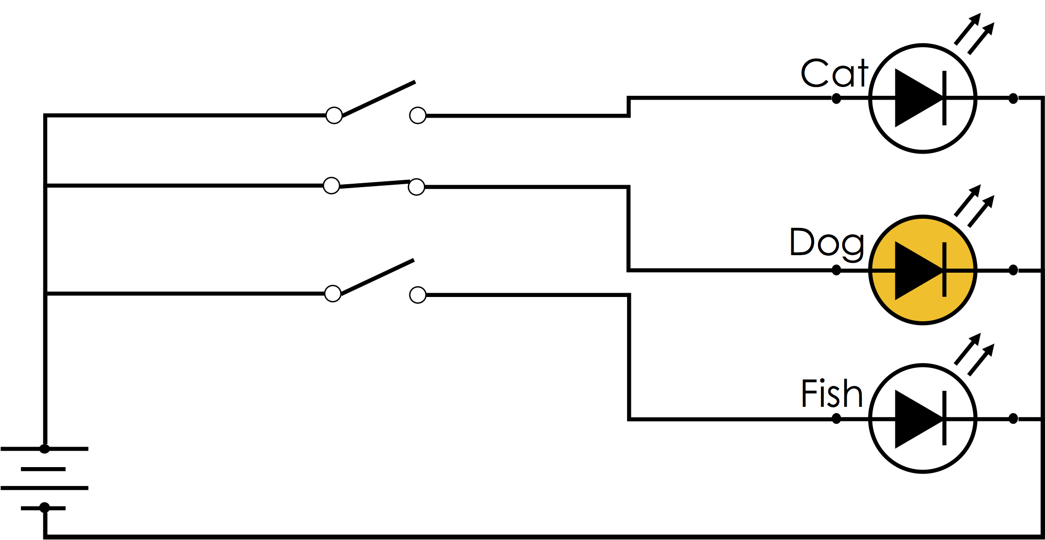
The term one-hot encoding comes from a digital circuit encoding of a categorical state as particular "hot" wire:
We can construct a one-hot (dummy) encoding of the origin column using the Pandas.get_dummies
function:
pd.get_dummies(data[['origin']])
origin_europe | origin_japan | origin_usa | |
---|---|---|---|
0 | 0 | 0 | 1 |
1 | 0 | 0 | 1 |
2 | 0 | 0 | 1 |
3 | 0 | 0 | 1 |
4 | 0 | 0 | 1 |
... | ... | ... | ... |
393 | 0 | 0 | 1 |
394 | 1 | 0 | 0 |
395 | 0 | 0 | 1 |
396 | 0 | 0 | 1 |
397 | 0 | 0 | 1 |
398 rows × 3 columns
Using the Pandas.get_dummies
, we can build a new feature function which extends our previous features with the additional dummy encoding columns.
def phi_with_origin(df):
Phi = phi_with_displacement(df)
return Phi.join(pd.get_dummies(df[['origin']]))
phi_with_origin(data).head()
cylinders | displacement | horsepower | weight | acceleration | model_year | horsepower_missing | displacement/cylinder | origin_europe | origin_japan | origin_usa | |
---|---|---|---|---|---|---|---|---|---|---|---|
0 | 8 | 307.0 | 130.0 | 3504 | 12.0 | 70 | 0.0 | 38.375 | 0 | 0 | 1 |
1 | 8 | 350.0 | 165.0 | 3693 | 11.5 | 70 | 0.0 | 43.750 | 0 | 0 | 1 |
2 | 8 | 318.0 | 150.0 | 3436 | 11.0 | 70 | 0.0 | 39.750 | 0 | 0 | 1 |
3 | 8 | 304.0 | 150.0 | 3433 | 12.0 | 70 | 0.0 | 38.000 | 0 | 0 | 1 |
4 | 8 | 302.0 | 140.0 | 3449 | 10.5 | 70 | 0.0 | 37.750 | 0 | 0 | 1 |
We fit a new model with the origin feature encoding:
model = LinearRegression()
model.fit(phi_with_origin(data), data[["mpg"]])
evaluate_model("cont.+(d/c)+o", model, phi_with_origin, models)
Root Mean Squared Error: 3.006188837672639
Unfortunately, the above feature function is not stable. For example, if we are given a single vehicle to make a prediction the model will fail:
try:
model.predict(phi_with_origin(data.head(1)))
except Exception as e:
print(e)
matmul: Input operand 1 has a mismatch in its core dimension 0, with gufunc signature (n?,k),(k,m?)->(n?,m?) (size 11 is different from 9)
To see why this fails look at the feature transformation for a single row:
phi_with_origin(data.head(1))
cylinders | displacement | horsepower | weight | acceleration | model_year | horsepower_missing | displacement/cylinder | origin_usa | |
---|---|---|---|---|---|---|---|---|---|
0 | 8 | 307.0 | 130.0 | 3504 | 12.0 | 70 | 0.0 | 38.375 | 1 |
The dummy columns are not created for the other categories.
There are a couple solutions. We could maintain a list of dummy columns and always add these columns. Alternatively, we could use a library function designed to solve this problem. The second option is much easier.
The scikit-learn library has a wide range feature transformations and a framework for composing them in reusable (stable) pipelines. Let's first look at a basic OneHotEncoder
transformation.
from sklearn.preprocessing import OneHotEncoder
oh_enc = OneHotEncoder()
We then fit that instance to some data. This is where we would determine the specific values that a categorical feature can take:
oh_enc.fit(data[['origin']])
OneHotEncoder()
Once we fit the transformation, we can then use it transform new data:
oh_enc.transform(data[['origin']].head())
<5x3 sparse matrix of type '<class 'numpy.float64'>' with 5 stored elements in Compressed Sparse Row format>
oh_enc.transform(data[['origin']].head()).todense()
matrix([[0., 0., 1.], [0., 0., 1.], [0., 0., 1.], [0., 0., 1.], [0., 0., 1.]])
We can also inspect the categories of the one-hot encoder:
oh_enc.get_feature_names()
array(['x0_europe', 'x0_japan', 'x0_usa'], dtype=object)
We can update our feature function to use the one-hot encoder instead.
def phi_with_origin(df):
Phi = phi_with_displacement(df)
dummies = pd.DataFrame(oh_enc.transform(df[['origin']]).todense(),
columns=oh_enc.get_feature_names(),
index = df.index)
return Phi.join(dummies)
phi_with_origin(data.head())
cylinders | displacement | horsepower | weight | acceleration | model_year | horsepower_missing | displacement/cylinder | x0_europe | x0_japan | x0_usa | |
---|---|---|---|---|---|---|---|---|---|---|---|
0 | 8 | 307.0 | 130.0 | 3504 | 12.0 | 70 | 0.0 | 38.375 | 0.0 | 0.0 | 1.0 |
1 | 8 | 350.0 | 165.0 | 3693 | 11.5 | 70 | 0.0 | 43.750 | 0.0 | 0.0 | 1.0 |
2 | 8 | 318.0 | 150.0 | 3436 | 11.0 | 70 | 0.0 | 39.750 | 0.0 | 0.0 | 1.0 |
3 | 8 | 304.0 | 150.0 | 3433 | 12.0 | 70 | 0.0 | 38.000 | 0.0 | 0.0 | 1.0 |
4 | 8 | 302.0 | 140.0 | 3449 | 10.5 | 70 | 0.0 | 37.750 | 0.0 | 0.0 | 1.0 |
model = LinearRegression()
model.fit(phi_with_origin(data), data[["mpg"]])
evaluate_model("cont.+(d/c)+o", model, phi_with_origin, models)
Root Mean Squared Error: 3.006188837672639
data[['name']]
name | |
---|---|
0 | chevrolet chevelle malibu |
1 | buick skylark 320 |
2 | plymouth satellite |
3 | amc rebel sst |
4 | ford torino |
... | ... |
393 | ford mustang gl |
394 | vw pickup |
395 | dodge rampage |
396 | ford ranger |
397 | chevy s-10 |
398 rows × 1 columns
The only remaining feature to encode is the vehicle name. Is there potentially signal in the vehicle name?
data[['name']].head(10)
name | |
---|---|
0 | chevrolet chevelle malibu |
1 | buick skylark 320 |
2 | plymouth satellite |
3 | amc rebel sst |
4 | ford torino |
5 | ford galaxie 500 |
6 | chevrolet impala |
7 | plymouth fury iii |
8 | pontiac catalina |
9 | amc ambassador dpl |
Encoding text can be challenging. The capturing the semantics and grammar of language in mathematical (vector) representations is an active area of research. State-of-the-art techniques often rely on neural networks trained on large collections of text. In this class, we will focus on basic text encoding techniques that are still widely used. If you are interested in learning more, checkout BERT Explained: A Complete Guide with Theory and Tutorial.
Here we present two widely used representations of text:
Both of these encoding strategies are related to the one-hot encoding with dummy features created for every word or sequence of words and with multiple dummy features having counts greater than zero.
The bag-of-words encoding is widely used and a standard representation for text in many of the popular text clustering algorithms. The following is a simple illustration of the bag-of-words encoding:
Notice
is
and about
that in isolation contain very little information about the meaning of the sentence. Here is a good list of stop-words in many languages. fun
, machines
, and learning
. Thought there are many possible meanings learning machines have fun learning or learning about machines is fun learning ...0
for every word that is not in each record would be inefficient. When professor Gonzalez was a graduate student at Carnegie Mellon University, he and several other computer scientists created the following art piece on display in the Gates Center:
Is this art or science?
Notice
We can use scikit-learn to construct a bag-of-words representation of text
frost_text = [x for x in """
Some say the world will end in fire,
Some say in ice.
From what Ive tasted of desire
I hold with those who favor fire.
""".split("\n") if len(x) > 0]
frost_text
['Some say the world will end in fire,', 'Some say in ice.', 'From what Ive tasted of desire', 'I hold with those who favor fire.']
from sklearn.feature_extraction.text import CountVectorizer
# Construct the tokenizer with English stop words
bow = CountVectorizer(stop_words="english")
# fit the model to the passage
bow.fit(frost_text)
CountVectorizer(stop_words='english')
# Print the words that are kept
print("Words:", list(enumerate(bow.get_feature_names())))
Words: [(0, 'desire'), (1, 'end'), (2, 'favor'), (3, 'hold'), (4, 'ice'), (5, 'ive'), (6, 'say'), (7, 'tasted'), (8, 'world')]
print("Sentence Encoding: \n")
# Print the encoding of each line
for (text, encoding) in zip(frost_text, bow.transform(frost_text)):
print(text)
print(encoding.todense())
print("------------------")
Sentence Encoding: Some say the world will end in fire, [[0 1 0 0 0 0 1 0 1]] ------------------ Some say in ice. [[0 0 0 0 1 0 1 0 0]] ------------------ From what Ive tasted of desire [[1 0 0 0 0 1 0 1 0]] ------------------ I hold with those who favor fire. [[0 0 1 1 0 0 0 0 0]] ------------------
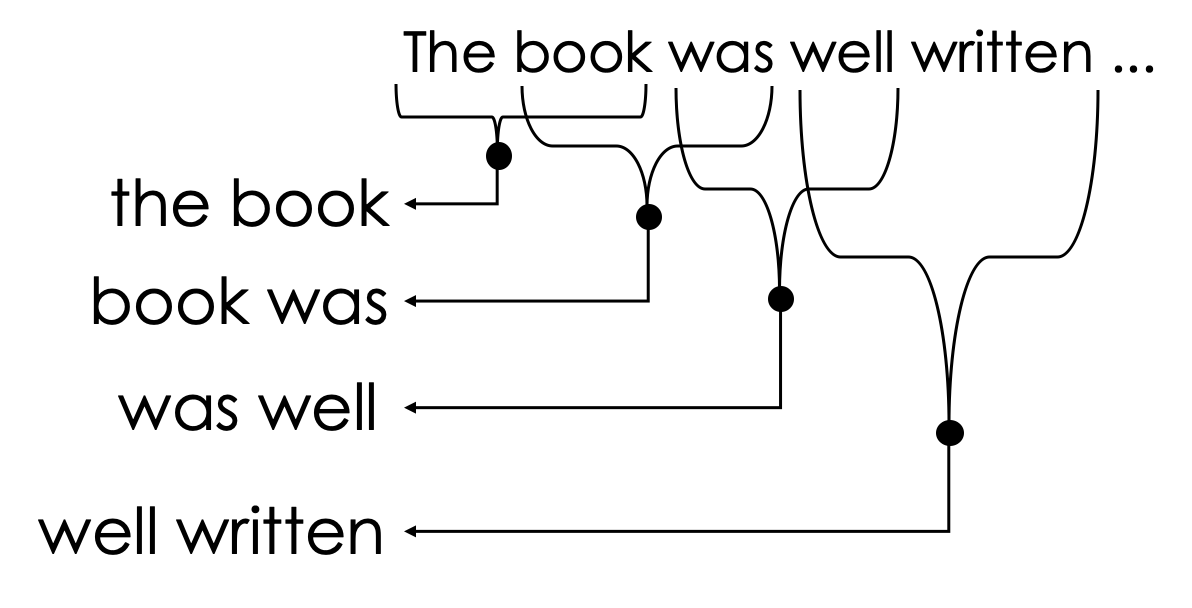
The n-gram encoding is a generalization of the bag-of-words encoding designed to capture information about word ordering. Consider the following passage of text:
The book was not well written but I did enjoy it.
If we re-arrange the words we can also write:
The book was well written but I did not enjoy it.
Moreover, local word order can be important when making decisions about text. The n-gram encoding captures local word order by defining counts over sliding windows. In the following example a bi-gram ($n=2$) encoding is constructed:
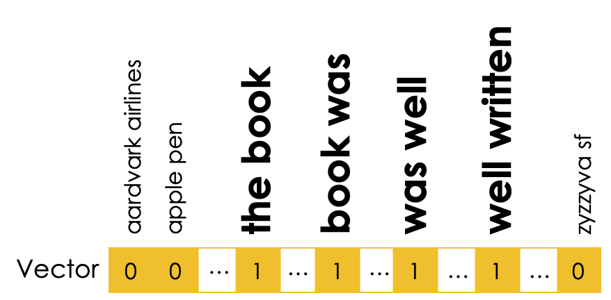
The above n-gram would be encoded in the sparse vector:
Notice that the n-gram captures key pieces of sentiment information: "well written"
and "not enjoy"
.
N-grams are often used for other types of sequence data beyond text. For example, n-grams can be used to encode genomic data, protein sequences, and click logs.
N-Gram Issues
# Construct the tokenizer with English stop words
bigram = CountVectorizer(ngram_range=(1, 2))
# fit the model to the passage
bigram.fit(frost_text)
CountVectorizer(ngram_range=(1, 2))
# Print the words that are kept
print("\nWords:",
list(zip(range(0,len(bigram.get_feature_names())), bigram.get_feature_names())))
Words: [(0, 'desire'), (1, 'end'), (2, 'end in'), (3, 'favor'), (4, 'favor fire'), (5, 'fire'), (6, 'from'), (7, 'from what'), (8, 'hold'), (9, 'hold with'), (10, 'ice'), (11, 'in'), (12, 'in fire'), (13, 'in ice'), (14, 'ive'), (15, 'ive tasted'), (16, 'of'), (17, 'of desire'), (18, 'say'), (19, 'say in'), (20, 'say the'), (21, 'some'), (22, 'some say'), (23, 'tasted'), (24, 'tasted of'), (25, 'the'), (26, 'the world'), (27, 'those'), (28, 'those who'), (29, 'what'), (30, 'what ive'), (31, 'who'), (32, 'who favor'), (33, 'will'), (34, 'will end'), (35, 'with'), (36, 'with those'), (37, 'world'), (38, 'world will')]
print("\nSentence Encoding: \n")
# Print the encoding of each line
for (text, encoding) in zip(frost_text, bigram.transform(frost_text)):
print(text)
print(encoding.todense())
print("------------------")
Sentence Encoding: Some say the world will end in fire, [[0 1 1 0 0 1 0 0 0 0 0 1 1 0 0 0 0 0 1 0 1 1 1 0 0 1 1 0 0 0 0 0 0 1 1 0 0 1 1]] ------------------ Some say in ice. [[0 0 0 0 0 0 0 0 0 0 1 1 0 1 0 0 0 0 1 1 0 1 1 0 0 0 0 0 0 0 0 0 0 0 0 0 0 0 0]] ------------------ From what Ive tasted of desire [[1 0 0 0 0 0 1 1 0 0 0 0 0 0 1 1 1 1 0 0 0 0 0 1 1 0 0 0 0 1 1 0 0 0 0 0 0 0 0]] ------------------ I hold with those who favor fire. [[0 0 0 1 1 1 0 0 1 1 0 0 0 0 0 0 0 0 0 0 0 0 0 0 0 0 0 1 1 0 0 1 1 0 0 1 1 0 0]] ------------------
We can add the text encoding features to our feature function:
bow = CountVectorizer()
bow.fit(data["name"])
def phi_with_name(df):
Phi = phi_with_origin(df)
bow_encoding = pd.DataFrame(
bow.transform(df['name']).todense(),
columns=bow.get_feature_names(),
index = df.index)
return Phi.join(bow_encoding)
Phi = phi_with_name(data)
Phi.head()
cylinders | displacement | horsepower | weight | acceleration | model_year | horsepower_missing | displacement/cylinder | x0_europe | x0_japan | ... | volkswagen | volvo | vw | wagon | woody | x1 | xe | yorker | zephyr | zx | |
---|---|---|---|---|---|---|---|---|---|---|---|---|---|---|---|---|---|---|---|---|---|
0 | 8 | 307.0 | 130.0 | 3504 | 12.0 | 70 | 0.0 | 38.375 | 0.0 | 0.0 | ... | 0 | 0 | 0 | 0 | 0 | 0 | 0 | 0 | 0 | 0 |
1 | 8 | 350.0 | 165.0 | 3693 | 11.5 | 70 | 0.0 | 43.750 | 0.0 | 0.0 | ... | 0 | 0 | 0 | 0 | 0 | 0 | 0 | 0 | 0 | 0 |
2 | 8 | 318.0 | 150.0 | 3436 | 11.0 | 70 | 0.0 | 39.750 | 0.0 | 0.0 | ... | 0 | 0 | 0 | 0 | 0 | 0 | 0 | 0 | 0 | 0 |
3 | 8 | 304.0 | 150.0 | 3433 | 12.0 | 70 | 0.0 | 38.000 | 0.0 | 0.0 | ... | 0 | 0 | 0 | 0 | 0 | 0 | 0 | 0 | 0 | 0 |
4 | 8 | 302.0 | 140.0 | 3449 | 10.5 | 70 | 0.0 | 37.750 | 0.0 | 0.0 | ... | 0 | 0 | 0 | 0 | 0 | 0 | 0 | 0 | 0 | 0 |
5 rows × 311 columns
model = LinearRegression()
model.fit(phi_with_name(data), data[["mpg"]])
evaluate_model("cont.+(d/c)+o+n", model, phi_with_name, models)
Root Mean Squared Error: 1.3566759335171261
Notice that as we added more features we were able to improve the accuracy of our model. This is not always a good thing and we will see the problems associated with this in a future lecture.
It is also worth noting that our feature functions each depended on the last and the in some cases we were converting sparse features to dense features. There is a better way to deal with feature pipelines using the scikit-learn pipelines module.