A Brief Introduction to Deep Learning

In this notebook, we provide a very quick (shallow?) introduction to neural networks and deep learning. We review the basic challenge of binary classification and linear decision functions and then show how features can be composed to express more complex decision surfaces. We then build a basic neural network to learn the feature functions and ultimately build more complex models for image classification.

Quick Review of Logistic Regression

We start by reviewing logistic regression. We construct a linearly separable data set and show how a logistic regression model fits this data.

We fit a logistic regression model.

The following block of code generates the prediction surface.

Notice that in the above plot we assign near zero probability of being a "plus" to the region on the left and a near one probability to the region on the right. Also notice that in the middle there is a transition region as the probability being a "plus" goes from zero to one.

Non-linearly Separable Data

We can modify the above data slightly to construct a data set that is no longer linearly separable. Can you find a decision line that would separate this data into "plus" and "circle" regions?

When we fit a logistic regression classifier to this data we no longer get an effective model.

How could we improve the classifier performance? One standard solution would be to leverage feature engineering. What feature transformations would help with this classification problem?

Manual Feature Engineering

Looking at the above figure it seems like the class depends on which quadrant the point is drawn from. We could one-hot encode the quadrant for each point a fit a model using these features instead of the original $X_1$ and $X_2$ features.

Again fitting the logistic regression model with these 4 new features.

Again we plot the decision surface.

This time we are able to accurately classify our data. The advantage of this approach is we are able to use domain knowledge and intuition in the design of our model. However, for many real-world problems, it may be very difficult to manually create these kinds of highly informative features. We would like to learn the features themselves. Notice that in the above example the features were also binary functions (just like the logistic regression function). Could we use logistic regression to build features as well as the final classifier? This is where neural networks begin.

Deep Learning

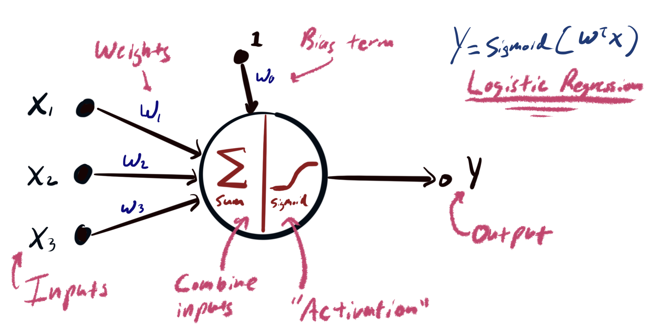
Classically, the standard approach to building models is to leverage domain knowledge to engineer features that capture the concepts we are trying to model. For example, if we want to detect cats in images we might want to look for edges, texture, and geometry that are unique to cats. These features are then fed into high-dimensional robust classification models like logistic regression.

Classic Feature Engineering Pipeline

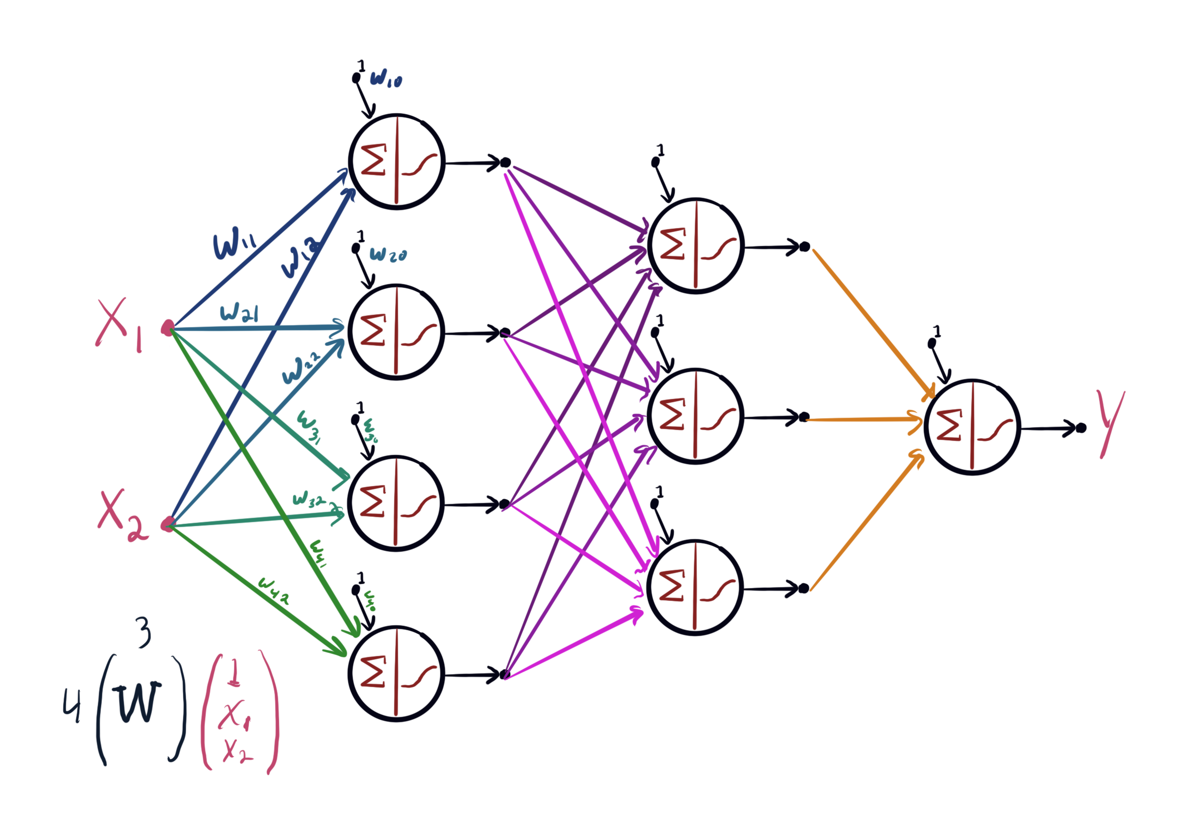
Descriptive features (e.g., cat textures) are often used as inputs to increasingly higher level features (e.g, cat ears). This composition of features results in "deep" pipelines of transformations producing increasingly more abstract feature concepts. However, manually designing these features is both challenging and may not actually produce the optimal feature representations.

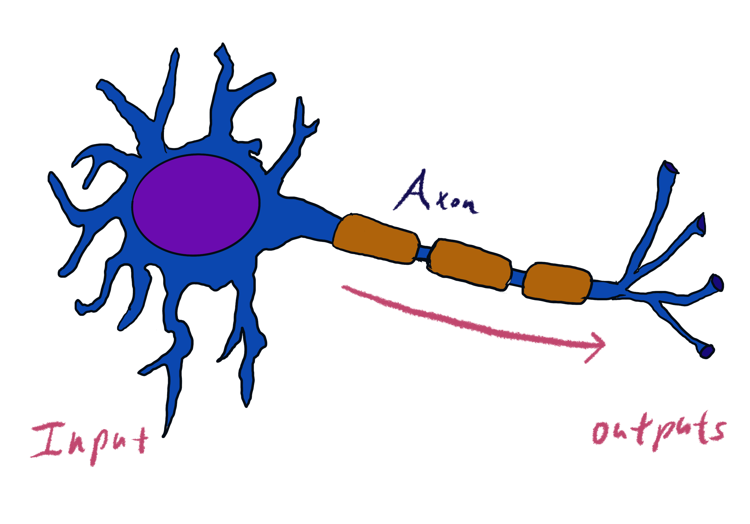
The idea in Deep Learning is to automatically learn entire pipelines of feature transformations and the resulting classifier from data. This is accomplished use neural networks. While neural networks were originally inspired by abstract models of neural computation, modern neural networks can be more accurately characterized as complex parameteric function expressed programatically as the composition of mathematical primitives. In the following, we will first describe a simple neural network pictorially and then programatically.

The Basic Neuron

Neural networks originated from a simple mathematical abstraction of a "neuron" as a computational device that accumulates input signals and produces an output. The following is a very simple diagram of a neuron. Conceptually signal arrive at the dendrites on the left and when the combine firing is sufficient to trigger an action potential across the axon an output is sent to the axon terminals on the right.

Simple Neuron

We can model this process (very abstractly) as a weighted summation of input values that is then transmitted to the output when the inputs exceed some threshold. This activation threshold could be modeled by a sigmoid function like is used in logistic regression. In this case, the behavior of this single artificial neuron is precisely the logistic regression model.

Artificial Neuron

We can combine these single artificial neurons into larger networks of neurons to express more complex functions. For example, the following network has multiple layers of neurons:

Artificial Neuron

This can be written as a mathematical expression:

\begin{align} A_1 & = \text{Sigmoid}(W X) \\ A_2 & = \text{Sigmoid}(U A_1) \\ \mathbb{P}(Y=1 \,|\, X) & = \text{Sigmoid}(V A_2) \end{align}

Here we assume that there is an implicit bias term added to each stage and the initial layer weight matrix $W\in \mathbb{R}^{4,3}$, the next layer weight matrix is in $U \in \mathbb{R}^{5,3}$, and the final weight matrix is in $V \in \mathbb{R}^{4,1}$. The vectors (often called activations) $A_1 \in \mathbb{R}^4$ and $A_1 \in \mathbb{R}^3$ correspond to the learned intermediate features.

Building a Neural Network

One of the significant innovations in deep learning is the introduction of libraries to simplify the design and training of neural networks. These libraries allow users to easily describe complex network structures and then automatically derivate optimization procedures to train these networks.

In the following we will use PyTorch to implement such a network.

Pytorch is a lot like Numpy in that you can express interesting computation interms of tensors:

Quick Introduction to Algorithmic Differentiation

In this lecture we are going to introduce PyTorch. PyTorch is sort of like learning how to use Thor's hammer, it is way overkill for basically everything you will do and is probably the wrong solution to most problems you will encounter. However, it also really powerful and will give you the skills needed to take on very challenging problems.

Defining a variable $\theta$ with an initial value 1.0

Suppose we compute the following value from our tensor theta

$$ z = \left(1 - log\left(1 + \exp(\theta) \right) \right)^2 $$

Notice that every derived value has an attached a gradient function that is used to compute the backwards path.

We can visualize these functions

These backward functions tell Torch how to compute the gradient via the chain rule. This is done by invoking backward on the computed value.

We can use item to extract a single value.

We can compare this witht he hand computed derivative:

\begin{align} \frac{\partial z}{\partial\theta} &= \frac{\partial}{\partial\theta}\left(1 - \log\left(1 + \exp(\theta)\right)\right)^2 \\ & = 2\left(1 - \log\left(1 + \exp(\theta)\right)\right)\frac{\partial}{\partial\theta} \left(1 - \log\left(1 + \exp(\theta)\right)\right)\\ & = 2\left(1 - \log\left(1 + \exp(\theta)\right)\right) (-1) \frac{\partial}{\partial\theta} \log\left(1 + \exp(\theta)\right) \\ & = 2\left(1 - \log\left(1 + \exp(\theta)\right)\right) \frac{-1}{1 + \exp(\theta)}\frac{\partial}{\partial\theta}\left(1 + \exp(\theta)\right) \\ & = 2\left(1 - \log\left(1 + \exp(\theta)\right)\right) \frac{-1}{1 + \exp(\theta)}\exp(\theta) \\ & = -2\left(1 - \log\left(1 + \exp(\theta)\right)\right) \frac{\exp(\theta)}{1 + \exp(\theta)} \end{align}

Image Classification

Evaluate the model: