In [1]:
# Support embedding YouTube Videos in Notebooks
from IPython.display import YouTubeVideo
In [2]:
YouTubeVideo("mYE0FhwHD-w")
Out[2]:

Pitfalls of Feature Engineering

In this notebook, we present three issues you might encounter in feature engineering:

  1. Redundant Features: When duplicate features are introduced this can create problems when solving the normal equation.
  2. Too many Features: When you add more features than you have data the solution to the normal equations becomes underdetermined.
  3. Overfitting: When improvements in the model or features introduced to fit the model to the available data result in poor predictions on new data.

The third issue overfitting will also be the focus on the next several lectures and is the fundamental challenge in modeling.

Imports

In this notebook we will be using the following packages:

In [3]:
import numpy as np
import pandas as pd
In [4]:
import plotly.offline as py
import plotly.express as px
import plotly.graph_objects as go
from plotly.subplots import make_subplots
import plotly.figure_factory as ff
import cufflinks as cf
cf.set_config_file(offline=True, sharing=False, theme='ggplot');
In [5]:
#import torch
from sklearn.linear_model import LinearRegression

Intro Video

The following video walk-through presents this notebook. I did not break it into sections but will try to do that in my next notebook.

In [6]:
YouTubeVideo("YHRG-OyFTLM")
Out[6]:


Toy Data and Model Setup

The following video provides an overview of the data and basic linear model setup.

In [7]:
YouTubeVideo("BJ270_CtU90")
Out[7]:

For this problem we will use a very simple toy dataset to help illustrate where things will fail.

In [8]:
data = pd.read_csv("data/train.csv")
data
Out[8]:
X Y
0 -2.647582 -3.158907
1 -2.051547 -2.862099
2 -1.810665 -0.412097
3 -1.312076 -1.534121
4 -0.789591 2.112187
5 -0.660964 -2.181700
6 -0.408638 1.281456
7 0.806148 4.273714
8 1.054880 2.450654
In [9]:
data_scatter = go.Scatter(x=data["X"], y=data["Y"], name="data", mode="markers")
go.Figure([data_scatter])


Fit a Basic Linear Model

For this notebook, we are going to implement the solution to the normal equations ourselves so that we can observe the resulting numerical issues.

In [10]:
from numpy.linalg import solve

def fit(X, Y):
    return solve(X.T @ X, X.T @ Y)

We will need to add a ones column to our feature matrix

In [11]:
def add_ones_column(data):
    n,_ = data.shape
    return np.hstack([np.ones((n,1)), data])

Constructing the original $\mathbb{X}$ and $\mathbb{Y}$ matrices

In [12]:
X = data[['X']].to_numpy()
Y = data[['Y']].to_numpy()
In [13]:
def phi_line(X):
    return add_ones_column(X)
In [14]:
Phi_line = phi_line(X)
Phi_line
Out[14]:
array([[ 1.        , -2.64758199],
       [ 1.        , -2.05154693],
       [ 1.        , -1.8106647 ],
       [ 1.        , -1.31207628],
       [ 1.        , -0.78959051],
       [ 1.        , -0.66096384],
       [ 1.        , -0.40863836],
       [ 1.        ,  0.80614815],
       [ 1.        ,  1.05487968]])

Fit the Model

Solving for $\hat{\theta}$ using our Phi matrix

In [15]:
theta_hat_line = fit(Phi_line, Y)
theta_hat_line
Out[15]:
array([[1.55382472],
       [1.79223445]])

Make Predictions

Make predictions at each of the original X values

In [16]:
def predict(theta, X):
    return X @ theta
In [17]:
data['Y_hat'] = predict(theta_hat_line, Phi_line)
data
Out[17]:
X Y Y_hat
0 -2.647582 -3.158907 -3.191263
1 -2.051547 -2.862099 -2.123028
2 -1.810665 -0.412097 -1.691311
3 -1.312076 -1.534121 -0.797724
4 -0.789591 2.112187 0.138693
5 -0.660964 -2.181700 0.369223
6 -0.408638 1.281456 0.821449
7 0.806148 4.273714 2.998631
8 1.054880 2.450654 3.444416
In [18]:
fig = go.Figure()
fig.add_trace(data_scatter)
basic_ols = go.Scatter(x=data['X'], y=data['Y_hat'], mode="lines", name="$y=mx+b$")
fig.add_trace(basic_ols)

Computing the Squared Loss

We compute the squared loss so we can compare with it later:

In [19]:
def squared_loss(Y, Y_hat):
    return np.mean((Y - Y_hat)**2)
In [20]:
loss_line = squared_loss(Y, data[['Y_hat']].to_numpy())
loss_line
Out[20]:
1.7725367178022595

Creating a Model Class

Because we are going to make a number of models. We can define a simple helper class to maintain our model.

In [21]:
class LinearModel:
    def __init__(self, phi):
        self.phi = phi
    def fit(self, X, Y):
        Phi = self.phi(X)
        self.theta_hat = solve(Phi.T @ Phi, Phi.T @ Y)
        return self.theta_hat
    def predict(self, X):
        Phi = self.phi(X)
        return Phi @ self.theta_hat
    def loss(self, X, Y):
        return np.mean((Y - self.predict(X))**2)

Building and training the model

In [22]:
model_line = LinearModel(phi_line)
model_line.fit(X,Y)
model_line.loss(X,Y)
Out[22]:
1.7725367178022595


The Issue with Redundant Feature

Redundant features occur when features are linear combinations of existing features.

In [23]:
YouTubeVideo("M11bB0Yd2is")
Out[23]:

Suppose we were to duplicate a feature. For example, suppose we copied the original value of $X$. Here we will make the features matrix:

\begin{align} \Phi = \left[1, X, X \right] \end{align}
In [24]:
def phi_dup(x):
    return add_ones_column(np.hstack([X, X]))
In [25]:
Phi_dup = phi_dup(X)
Phi_dup
Out[25]:
array([[ 1.        , -2.64758199, -2.64758199],
       [ 1.        , -2.05154693, -2.05154693],
       [ 1.        , -1.8106647 , -1.8106647 ],
       [ 1.        , -1.31207628, -1.31207628],
       [ 1.        , -0.78959051, -0.78959051],
       [ 1.        , -0.66096384, -0.66096384],
       [ 1.        , -0.40863836, -0.40863836],
       [ 1.        ,  0.80614815,  0.80614815],
       [ 1.        ,  1.05487968,  1.05487968]])

Note that any feature that is a linear combination of other features would be problematic. If we attempt to solve for the new $\hat{\theta}$ for this revised model we get:

In [26]:
try:
    theta_hat_dup = solve(Phi_dup.T @ Phi_dup, Phi_dup.T @ Y)
    print(theta_hat_dup)
except np.linalg.LinAlgError as err:
    print(err)
Singular matrix

The above fails because the $\Phi^T \Phi$ matrix is no longer full rank and we cannot solve for $\theta$ in the system of linear equations:

$$ \Phi^T \Phi \theta = \Phi^T Y $$

We can actually check the rank of this 3x3 matrix:

In [27]:
Phi_dup.T @ Phi_dup
Out[27]:
array([[ 9.        , -7.82003478, -7.82003478],
       [-7.82003478, 19.20854372, 19.20854372],
       [-7.82003478, 19.20854372, 19.20854372]])
In [28]:
from numpy.linalg import matrix_rank
matrix_rank(Phi_dup.T @ Phi_dup)
Out[28]:
2

There are actually infinitely many possible optimal solutions. We can consider the two extreme parameterizations where we ignore (set the coefficient to zero) one or the other redundant feature:

In [29]:
theta_a = np.array([[theta_hat_line[0,0], theta_hat_line[1,0], 0]]).T
theta_a
Out[29]:
array([[1.55382472],
       [1.79223445],
       [0.        ]])
In [30]:
theta_b = np.array([[theta_hat_line[0,0], 0, theta_hat_line[1,0]]]).T
theta_b
Out[30]:
array([[1.55382472],
       [0.        ],
       [1.79223445]])

Then we can examine the squared loss for many possible convex combinations of the two parameters.

In [31]:
def convex_comb(theta_a, theta_b, alpha):
    return alpha * theta_a + (1-alpha) * theta_b
In [32]:
[squared_loss(predict(convex_comb(theta_a, theta_b, a), Phi_dup), Y) 
 for a in np.linspace(0, 1, 10)]
Out[32]:
[1.7725367178022595,
 1.7725367178022595,
 1.7725367178022597,
 1.7725367178022595,
 1.7725367178022593,
 1.7725367178022593,
 1.7725367178022593,
 1.7725367178022595,
 1.7725367178022593,
 1.7725367178022595]

They are equivalent up to numerical precision.


Too Many Features

In the basic formulation of least squares regression we assumed that there was far more data than features. What if this is not the case? Let's examine what happens when we add too many features.

In [33]:
YouTubeVideo("iwbqbPg740I")
Out[33]:

To illustrate this, let's introduce a feature that is 1 when we are near a particular location and decreases quickly as we move away. This is actually called a radial basis function. These are used when you might imagine something happens near a particular value. For example, if you were trying to predict when someone asks their Smart Alarm to Snooze you might place radial basis functions around common hours (e.g., 6AM, 7AM, and 8AM).

The following block of code creates a single radial basis function feature.

In [34]:
def rbf_feature(loc, x, beta=0.1):
    return np.exp(-((loc - x)**2)/beta)

Notice that there is an additional $\beta$ hyper-parameter. This hyper-parameter determines the width of each bump.

In [35]:
z = np.linspace(-3,3,300)
fig = go.Figure()
fig.add_trace(go.Scatter(x=z, y=rbf_feature(0, z, beta=0.1), mode="lines", name=r"$\beta=0.1$"))
fig.add_trace(go.Scatter(x=z, y=rbf_feature(0, z, beta=1.), mode="lines", name=r"$\beta=1$"))
fig.add_trace(go.Scatter(x=z, y=rbf_feature(0, z, beta=2.), mode="lines", name=r"$\beta=2$"))

We can place these radial basis function features at different locations along the x-axis to implement multiple features.

In [36]:
def phi_rbf(locations, X):
    return np.hstack([rbf_feature(loc, X) for loc in locations])

Suppose we start by placing four bumps at a few locations along the x-axis:

In [37]:
four_bump_locations = [-2, -1, 0, 1]
In [38]:
Phi_rbf4 = phi_rbf(four_bump_locations, X)
Phi_rbf4
Out[38]:
array([[1.50914885e-02, 1.62540481e-12, 3.60828942e-31, 1.65101703e-58],
       [9.73779036e-01, 1.57682910e-05, 5.26282822e-19, 3.62046310e-41],
       [6.98738603e-01, 1.39931489e-03, 5.77599135e-15, 4.91414509e-35],
       [8.80539739e-03, 3.77601428e-01, 3.33755673e-08, 6.08042656e-24],
       [4.33700607e-07, 6.42286031e-01, 1.96054712e-03, 1.23349234e-14],
       [1.63313665e-08, 3.16809337e-01, 1.26672920e-02, 1.04395061e-12],
       [1.00412569e-11, 3.02855088e-02, 1.88274729e-01, 2.41245682e-09],
       [6.33318729e-35, 6.80096730e-15, 1.50532198e-03, 6.86749706e-01],
       [2.95379279e-41, 4.58968617e-19, 1.46992886e-05, 9.70331226e-01]])

Building a model

In [39]:
model_rbf4 = LinearModel(lambda X: phi_rbf(four_bump_locations, X))
In [40]:
model_rbf4.fit(X, Y)
Out[40]:
array([[-2.18307698],
       [ 0.10089646],
       [ 6.15481238],
       [ 3.75501581]])

Predicting the data and computing the loss:

In [41]:
model_rbf4.loss(X, Y)
Out[41]:
3.0708837738803343

Visualizing the Model

To visualize this model we will want to make predictions at more locations along the x-axis. We will call all these locations x_test (that is where we want to test the model).

In [42]:
X_test = np.expand_dims(np.linspace(X.min()-1, X.max()+1, 200), 1)
In [43]:
fig = go.Figure([data_scatter])

# Redraw the line plot so it extends out beyond data.
line_plot = go.Scatter(
    x=X_test.flatten(), 
    y=model_line.predict(X_test).flatten(),
    mode="lines", name="$y=mx+b$")
fig.add_trace(line_plot)

# Draw the new model
phi_rbf4_plot = go.Scatter(x=X_test.flatten(), 
                           y=model_rbf4.predict(X_test).flatten(),
                           mode="lines", name="4 RBF Features")
fig.add_trace(phi_rbf4_plot)

# Draw the Bumps
for b in four_bump_locations:
    fig.add_trace(go.Scatter(x=X_test.flatten(), 
                             y=rbf_feature(b, X_test).flatten(), 
                             name="Bump @ " + str(b),
                             line=dict(dash="longdash")))

fig

Notice that the Four RBF function model doesn't really follow the linear trend in the data. Let's add a the line features as well.

In [44]:
def phi_line_rbf(locations, X):
    return np.hstack([phi_line(X), phi_rbf(locations, X)])

As before we create the transformed features:

In [45]:
phi_line_rbf(four_bump_locations, X)
Out[45]:
array([[ 1.00000000e+00, -2.64758199e+00,  1.50914885e-02,
         1.62540481e-12,  3.60828942e-31,  1.65101703e-58],
       [ 1.00000000e+00, -2.05154693e+00,  9.73779036e-01,
         1.57682910e-05,  5.26282822e-19,  3.62046310e-41],
       [ 1.00000000e+00, -1.81066470e+00,  6.98738603e-01,
         1.39931489e-03,  5.77599135e-15,  4.91414509e-35],
       [ 1.00000000e+00, -1.31207628e+00,  8.80539739e-03,
         3.77601428e-01,  3.33755673e-08,  6.08042656e-24],
       [ 1.00000000e+00, -7.89590508e-01,  4.33700607e-07,
         6.42286031e-01,  1.96054712e-03,  1.23349234e-14],
       [ 1.00000000e+00, -6.60963845e-01,  1.63313665e-08,
         3.16809337e-01,  1.26672920e-02,  1.04395061e-12],
       [ 1.00000000e+00, -4.08638356e-01,  1.00412569e-11,
         3.02855088e-02,  1.88274729e-01,  2.41245682e-09],
       [ 1.00000000e+00,  8.06148154e-01,  6.33318729e-35,
         6.80096730e-15,  1.50532198e-03,  6.86749706e-01],
       [ 1.00000000e+00,  1.05487968e+00,  2.95379279e-41,
         4.58968617e-19,  1.46992886e-05,  9.70331226e-01]])
In [46]:
model_line_rbf4 = LinearModel(lambda X: phi_line_rbf(four_bump_locations, X))
model_line_rbf4.fit(X,Y)
Out[46]:
array([[-0.79713927],
       [ 1.00575004],
       [ 1.06793407],
       [ 3.52182177],
       [12.10002781],
       [ 3.56283746]])

Predicting the data and computing the loss:

In [47]:
model_line_rbf4.loss(X,Y)
Out[47]:
1.6298029998184385

Visualizing the Model

Evaluating the model at X_test locations.

In [48]:
fig = go.Figure([data_scatter, line_plot, phi_rbf4_plot])
# Draw the new model
phi_line_rbf4_plot = go.Scatter(x=X_test.flatten(), 
                                y=model_line_rbf4.predict(X_test).flatten(), 
                                mode="lines", name="Line + 4 RBF Features")
fig.add_trace(phi_line_rbf4_plot)
fig

Notice above that the newest model which combines RBF features and the line features better follows the trends in the data.

Let's try to add many more features.

Let's place 20 evenly spaced bumps between -3 and 3.

In [49]:
many_bump_locations = np.linspace(-3, 3, 20)

Notice the shape of our new matrix

In [50]:
Phi_line_rbf20 = phi_line_rbf(many_bump_locations, X)
Phi_line_rbf20.shape
Out[50]:
(9, 22)

Let's fit these 9 data points to a 22 feature linear model:

In [51]:
model_line_rbf20 = LinearModel(lambda X: phi_line_rbf(many_bump_locations, X))
In [52]:
model_line_rbf20.fit(X,Y)
Out[52]:
array([[-1.21261704e+00],
       [-7.94614797e-01],
       [ 1.18941833e+01],
       [-1.64096545e+01],
       [ 1.98208474e+01],
       [-1.33982127e+01],
       [ 9.13273350e+00],
       [-1.27346634e+01],
       [ 1.29861322e+01],
       [ 5.60379455e-01],
       [-7.62337236e+00],
       [ 2.13496508e+01],
       [-5.30723394e+01],
       [ 5.07016752e+00],
       [ 2.57836126e+00],
       [ 4.66667966e+00],
       [ 3.33106747e+01],
       [ 1.90500013e+02],
       [-1.79710226e+05],
       [ 7.21986916e+07],
       [-8.06865309e+11],
       [-9.22131511e+16]])

That worked!? Should it have worked? Recall we are solving:

$$ \Phi^T \Phi \hat{\theta} = \Phi^T \mathbb{Y} $$

There should be more than one solution since we have way more variables than we have equations. Put another way the inverse operation here should not be well defined:

$$ \hat{\theta} = \left(\Phi^T \Phi \right)^{-1} \Phi^T \mathbb{Y} $$

We can examine the rank and inverse of this matrix:

In [53]:
A = Phi_line_rbf20.T @ Phi_line_rbf20
A.shape
Out[53]:
(22, 22)
In [54]:
matrix_rank(A)
Out[54]:
9

Numpy uses iterative algorithms to invert matrices and does not necessarily check that a solution was found.

In [55]:
from numpy.linalg import inv
inv(A) @ A
Out[55]:
array([[-7.04465209e+00, -7.20183831e+00,  2.90737653e-01,
         8.23733930e-01,  5.54302693e-01,  1.56416999e-01,
         2.54800373e-02, -3.42212522e-01, -8.37484097e-01,
        -1.93705683e+00, -1.82818971e+00, -5.45484559e-01,
        -5.32567553e-02, -4.40609592e-01, -3.55498246e+00,
        -5.51501849e+00, -1.43733576e+00, -5.21595236e-02,
        -2.54826738e-04, -1.74303496e-07, -1.57742249e-11,
        -1.96282449e-16],
       [ 1.12596552e+01,  4.87393027e+00, -1.36426899e-01,
        -3.33611951e-01, -2.12760167e-01,  6.68346678e-02,
         7.76905485e-01,  1.06379792e+00,  1.23658799e+00,
         2.45936832e+00,  2.20508211e+00,  7.45747409e-01,
         6.19048025e-02,  4.73554262e-01,  3.72801651e+00,
         6.57182511e+00,  1.67115638e+00,  6.18163888e-02,
         3.04623996e-04,  2.03595443e-07,  1.88262552e-11,
         2.33712687e-16],
       [ 4.83053968e+11, -8.54840135e+11,  3.97078129e+10,
         1.37512819e+11,  1.04201269e+11,  1.54313032e+11,
         1.27756790e+11,  6.26245032e+10,  4.09560640e+10,
         6.05043902e+10,  1.05064680e+11,  4.73626079e+10,
         2.45889820e+09, -2.03143618e+10, -4.12580229e+10,
         2.25893872e+10,  1.18599905e+10,  4.77134876e+08,
         2.41676225e+06,  1.64093384e+03,  1.51154815e-01,
         1.89361454e-06],
       [-1.45421354e+11,  2.57346113e+11, -1.19538727e+10,
        -4.13976648e+10, -3.13693599e+10, -4.64552968e+10,
        -3.84606512e+10, -1.88528483e+10, -1.23296567e+10,
        -1.82146006e+10, -3.16292747e+10, -1.42583082e+10,
        -7.40240421e+08,  6.11555563e+09,  1.24205731e+10,
        -6.80040969e+09, -3.57039251e+09, -1.43639168e+08,
        -7.27554722e+05, -4.93995293e+02, -4.55044348e-02,
        -5.70063610e-07],
       [ 8.69709348e+09, -1.53911108e+10,  7.14922894e+08,
         2.47586185e+09,  1.87609939e+09,  2.77833698e+09,
         2.30020493e+09,  1.12753041e+09,  7.37404293e+08,
         1.08936653e+09,  1.89161925e+09,  8.52724772e+08,
         4.42699029e+07, -3.65754235e+08, -7.42869449e+08,
         4.06642352e+08,  2.13515402e+08,  8.58992889e+06,
         4.35093896e+04,  2.95420254e+01,  2.72126733e-03,
         3.40910837e-08],
       [-5.95402358e+08,  1.05376080e+09, -4.89464723e+07,
        -1.69507345e+08, -1.28444597e+08, -1.90213835e+08,
        -1.57479823e+08, -7.71959328e+07, -5.04882881e+07,
        -7.45860020e+07, -1.29497681e+08, -5.83736769e+07,
        -3.03031850e+06,  2.50419133e+07,  5.08730400e+07,
        -2.78142618e+07, -1.46111134e+07, -5.87845059e+05,
        -2.97755539e+03, -2.02170527e+00, -1.86229698e-04,
        -2.33302055e-09],
       [ 1.50521068e+07, -2.66885273e+07,  1.23903464e+06,
         4.29090401e+06,  3.25108900e+06,  4.81384713e+06,
         3.98567824e+06,  1.95454494e+06,  1.27956743e+06,
         1.89013560e+06,  3.27239785e+06,  1.47356946e+06,
         7.63842799e+04, -6.34430584e+05, -1.29527510e+06,
         6.89352769e+05,  3.65911042e+05,  1.47362841e+04,
         7.46560607e+01,  5.06919829e-02,  4.66953662e-06,
         5.84984129e-11],
       [-1.46536548e+05,  2.68734560e+05, -1.23618865e+04,
        -4.28068920e+04, -3.23679667e+04, -4.77973673e+04,
        -3.96203220e+04, -1.95747789e+04, -1.30463930e+04,
        -1.92435400e+04, -3.15959744e+04, -1.39442587e+04,
        -7.02259982e+02,  6.41877238e+03,  1.42737001e+04,
        -4.18655771e+03, -2.92699334e+03, -1.20583254e+02,
        -6.13416289e-01, -4.16861756e-04, -3.84066398e-08,
        -4.81159911e-13],
       [ 2.49379214e+03, -4.80819995e+03,  2.17738249e+02,
         7.53463369e+02,  5.66446243e+02,  8.29436470e+02,
         6.91065520e+02,  3.54531942e+02,  2.53840340e+02,
         3.76201315e+02,  5.12784054e+02,  2.08997671e+02,
         9.79235254e+00, -1.07514760e+02, -2.71203689e+02,
        -5.82579457e+00,  2.80021691e+01,  1.24643483e+00,
         6.42347013e-03,  4.36603197e-06,  4.02166632e-10,
         5.05361119e-15],
       [-2.76071613e+01,  1.75677052e+01, -1.34781262e+00,
        -4.44329837e+00, -2.75948837e+00, -2.49430307e+00,
        -2.76309199e+00, -3.84025197e+00, -5.88977117e+00,
        -9.36388701e+00,  2.21456925e+00,  3.84185067e+00,
         1.70822024e-01, -3.91974695e+00, -1.20422341e+01,
        -6.07999918e+00, -6.53975233e-01, -1.57679636e-02,
        -7.70662317e-05, -4.38172357e-08, -4.10129034e-12,
        -5.21020592e-17],
       [ 1.24698407e+01,  1.19562956e+02, -4.18475414e+00,
        -1.44437685e+01, -1.06955654e+01, -1.49454788e+01,
        -1.17766565e+01, -3.37318280e+00,  3.59632577e-01,
         4.15381316e+00, -1.78766301e+00, -2.73468322e+00,
         7.55511759e-02,  7.56102944e+00,  3.33232052e+01,
         3.49156004e+01,  7.66373696e+00,  2.65666531e-01,
         1.30714767e-03,  8.74539908e-07,  8.12741657e-11,
         1.01778421e-15],
       [-1.21681151e+01, -4.92089275e+01,  2.45939532e+00,
         8.19883245e+00,  5.48357413e+00,  6.34719572e+00,
         4.22363397e+00, -7.31013295e-01, -2.80040781e+00,
        -5.59289637e+00, -2.49415676e+00,  6.00445480e-01,
        -1.45950899e-02, -1.77910701e+00, -1.13086187e+01,
        -1.66927902e+01, -4.13707327e+00, -1.45319297e-01,
        -7.22269066e-04, -4.86136611e-07, -4.70017700e-11,
        -5.76995832e-16],
       [-9.55791697e+01, -1.30134284e+03,  3.42639877e+01,
         1.22885236e+02,  9.06165109e+01,  1.56549903e+02,
         1.44453575e+02,  8.17530404e+01,  5.01730302e+01,
         3.07929191e+01,  9.38264422e+01,  3.73910131e+01,
        -1.04634907e+00, -1.01477877e+02, -4.09459182e+02,
        -3.63510832e+02, -7.42129700e+01, -2.51589586e+00,
        -1.26192033e-02, -8.36387381e-06, -7.62563395e-10,
        -9.48087694e-15],
       [-1.53432266e+01,  2.92559136e+01, -6.96834045e-01,
        -3.36506021e+00, -3.17018228e+00, -5.77512746e+00,
        -4.04327757e+00, -4.83181255e+00, -2.43519683e+00,
         4.80439569e-01, -2.73525459e+00, -2.38173286e+00,
        -2.09166200e-01,  2.06304328e-02, -2.48313991e-01,
         5.17999418e-01,  3.66772929e-02,  1.17027622e-02,
         1.10110500e-04,  7.58791909e-08,  3.41661597e-12,
         3.83483620e-17],
       [-3.19552523e+00,  1.39268045e+01, -6.52529303e-01,
        -1.86520934e+00, -1.31206388e+00, -1.42043047e+00,
        -1.66887767e+00, -2.99547549e-01, -1.44785275e-01,
        -7.23993936e-01, -5.25137984e-01, -4.58350686e-02,
         3.29578870e-02,  7.25640400e-01,  3.00494730e+00,
         1.33389972e+00,  1.30622249e-01,  4.11974584e-03,
         1.41456209e-05,  1.09787562e-08,  3.87652197e-13,
         8.82170191e-18],
       [ 2.16459290e+01,  2.87227392e+00,  6.34446365e-01,
         2.10221666e+00,  1.71655658e+00,  2.24236180e+00,
         1.59091146e+00,  1.15602361e+00,  1.02945999e+00,
         1.10472001e+00,  6.03021731e-01,  5.02124551e-01,
         1.45809027e-01,  2.76346250e+00,  1.19732575e+01,
         1.04799290e+01,  2.11204727e+00,  6.00056660e-02,
         3.48917501e-04,  2.37593919e-07,  2.50872008e-11,
         3.20732518e-16],
       [-1.27739822e+02,  1.23373986e+02, -8.63352837e+00,
        -3.07846044e+01, -2.18279403e+01, -2.49428837e+01,
        -2.11928089e+01, -1.01448882e+01, -1.18154501e+01,
        -1.94735667e+01, -1.86993639e+01, -5.91296434e+00,
        -6.42006366e-01, -6.05168925e+00, -2.58423860e+01,
        -2.21386777e+01, -4.41544135e+00, -1.17214201e-01,
        -7.60956002e-04, -5.96032076e-07, -5.65822748e-11,
        -4.20140421e-16],
       [ 1.43520505e+03,  4.36593087e+03, -4.17039991e+01,
        -1.72551997e+02, -1.92175929e+02, -4.73723088e+02,
        -4.42593744e+02, -1.84339320e+02, -7.46631183e+01,
         4.98496353e+01,  8.34462636e+01,  4.79533272e+01,
         1.96249207e+01,  3.62581682e+02,  1.76262408e+03,
         1.73193546e+03,  3.94436645e+02,  1.30559611e+01,
         6.68823839e-02,  4.29579006e-05,  4.24488149e-09,
         4.88685685e-14],
       [-1.78549053e+05, -1.05184891e+06,  2.19787750e+04,
         6.54961465e+04,  6.01573193e+04,  1.08604237e+05,
         1.14667845e+05,  5.22960959e+04,  3.26764993e+04,
         4.06735042e+04,  4.00495806e+04,  4.58707896e+03,
        -2.97149998e+03, -8.76615410e+04, -3.68430987e+05,
        -3.43590498e+05, -7.82606658e+04, -2.86871279e+03,
        -1.34433282e+01, -8.69542136e-03, -8.19968815e-07,
        -1.03825596e-11],
       [-1.30317600e+08,  8.11691723e+08, -2.61841137e+07,
        -7.89310577e+07, -7.58724667e+07, -1.17275260e+08,
        -1.10343044e+08, -7.82192642e+07, -4.18827546e+07,
        -1.07460980e+07, -1.35160254e+07, -4.54162402e+06,
        -1.49032041e+04,  1.06868917e+07,  1.07659061e+08,
         1.52263551e+08,  4.26689716e+07,  1.55322404e+06,
         7.25485047e+03,  6.17429590e+00,  5.17254864e-04,
         6.47488554e-09],
       [ 1.98552610e+12, -1.22953240e+13,  4.44367944e+11,
         1.48918463e+12,  1.17156573e+12,  1.63992701e+12,
         1.39395562e+12,  9.00887236e+11,  5.16309913e+11,
         2.32924683e+11,  2.80929885e+11,  8.52032985e+10,
         6.29059964e+08, -1.64789083e+11, -1.74465762e+12,
        -2.50830055e+12, -6.27460059e+11, -2.40261201e+10,
        -1.23340148e+08, -8.16202674e+04, -7.34868351e+00,
        -8.19329922e-05],
       [ 9.53941530e+16, -5.28583317e+17,  2.02494078e+16,
         7.48966681e+16,  5.52079796e+16,  8.79707193e+16,
         6.90452342e+16,  2.72706567e+16,  1.50423957e+16,
         1.26800131e+16,  1.13765314e+16, -1.00484760e+15,
        -1.07746884e+15, -1.92164902e+16, -7.79473553e+16,
        -6.03620370e+16, -1.42946628e+16, -4.93267215e+14,
        -2.60892193e+12, -1.98249789e+09, -1.40465621e+05,
        -1.60412862e+00]])

By comparison if we look at something that was more appropriate:

In [56]:
B = model_rbf4.phi(X).T @ model_rbf4.phi(X)
inv(B) @ B
Out[56]:
array([[ 1.00000000e+00, -4.33680869e-19,  1.35525272e-20,
         2.11758237e-22],
       [ 8.67361738e-19,  1.00000000e+00, -3.46944695e-18,
         0.00000000e+00],
       [-4.33680869e-19, -5.55111512e-17,  1.00000000e+00,
        -3.46944695e-18],
       [ 2.11758237e-22,  2.71050543e-20, -2.16840434e-19,
         1.00000000e+00]])

We can still use the model to make predictions since the algorithm did return a $\hat{\theta}$

In [57]:
fig = go.Figure([data_scatter, line_plot, phi_rbf4_plot, phi_line_rbf4_plot])
# Draw the new model
phi_line_rbf20_plot = go.Scatter(
    x=X_test.flatten(), 
    y=model_line_rbf20.predict(X_test).flatten(), 
    mode="lines", name="Line + 20 RBF Features")
fig.add_trace(phi_line_rbf20_plot)
fig.update_yaxes(range=[-5,10])
fig

Notice that despite the solution to the linear systems being not well posed, we were able to find a model that does appear to minimize the loss. When we cover regularization, we will return to how we can effectively train models when there are more features than data.


Overfitting

One of the big challenges is machine learning and statistics is building models that generalize beyond the data. Unfortunately, when building our models the data is all we have and we design our models to reflect the patterns in our data. However, it is possible to go too far.

In [58]:
YouTubeVideo("b6l9eVGERxY")
Out[58]:

Using our earlier example with with a more reasonable number of features

In [59]:
bump_locations7 = [-2, -1.5, -1, -0.5, 0, 0.5, 1]
In [60]:
Phi_line_rbf7 = phi_line_rbf(bump_locations7, X)
Phi_line_rbf7.shape
Out[60]:
(9, 9)

Notice that we have 9 data points and 9 features (2 linear model features and 7 RBF features).

In [61]:
model_line_rbf7 = LinearModel(lambda X: phi_line_rbf(bump_locations7, X))
model_line_rbf7.fit(X, Y)
Out[61]:
array([[ 183.07678483],
       [  70.11647712],
       [ -39.52065106],
       [ -75.53048989],
       [-103.34145656],
       [-135.26338052],
       [-135.66185885],
       [-152.97528896],
       [-255.11939771]])

Predicting the data and computing the loss:

In [62]:
model_line_rbf7.loss(X, Y)
Out[62]:
1.9925944342240575e-23

Visualizing the Model

In [63]:
fig = go.Figure([data_scatter, line_plot, phi_rbf4_plot, phi_line_rbf4_plot])
# Draw the new model
phi_line_rbf7_plot = go.Scatter(
    x=X_test.flatten(), 
    y=model_line_rbf7.predict(X_test).flatten(), 
    mode="lines", name="Line + 7 RBF Features")
fig.add_trace(phi_line_rbf7_plot)
fig.update_yaxes(range=[-10,20])
fig

Did we minimize the error? Let's compare the models:

In [64]:
models = [model_line, model_rbf4, model_line_rbf4, model_line_rbf7]
model_names = ["Line", "4 RBF", "Line + 4 RBF", "Line + 7 RBF"]
train_loss = [m.loss(X, Y) for m in models]
In [65]:
go.Figure([go.Bar(x=model_names, y=train_loss)])

While we minimized the training loss with the latest model it may not have been our "best" model. Why?

Examining New (Test) Data

To see why the models we developed above may actually be bad models despite minimizing the loss, we collect some more data from the same underlying process:

In [66]:
test_data = pd.read_csv("data/test.csv")
test_data
Out[66]:
X Y
0 -2.972389 -4.788094
1 -2.897078 -5.332368
2 -2.872904 -4.580639
3 -2.828057 -8.233739
4 -2.773864 -4.943137
... ... ...
95 1.753572 3.038685
96 1.828160 4.517537
97 1.847923 5.309920
98 1.849549 5.197142
99 1.934435 6.357799

100 rows × 2 columns

Plotting this new data (in red) on top of the old data we see that while the more complex RBF model fit the original data perfectly, it does not fit the new

In [67]:
test_data_scatter = go.Scatter(name = "Test Data", x = test_data['X'], y = test_data['Y'], 
                       mode = 'markers', marker=dict(symbol="cross", color="red"))
fig = go.Figure([data_scatter, test_data_scatter, line_plot, phi_rbf4_plot, phi_line_rbf4_plot, phi_line_rbf7_plot])
fig.update_yaxes(range=[-10,20])
fig

How do we perform on the new data? Computing the loss from before and after.

In [68]:
X_test = test_data[["X"]].to_numpy()
Y_test = test_data[["Y"]].to_numpy()
In [69]:
test_loss = [m.loss(X_test, Y_test) for m in models]
test_loss
Out[69]:
[3.330941371262085, 11.451610137092905, 13.580776824816382, 10203.10808252144]
In [70]:
fig = go.Figure([go.Bar(x=model_names, y=train_loss, name="Train Loss"), 
           go.Bar(x=model_names, y=test_loss, name="Test Loss")])
fig.update_yaxes(range=[-0.1,15])

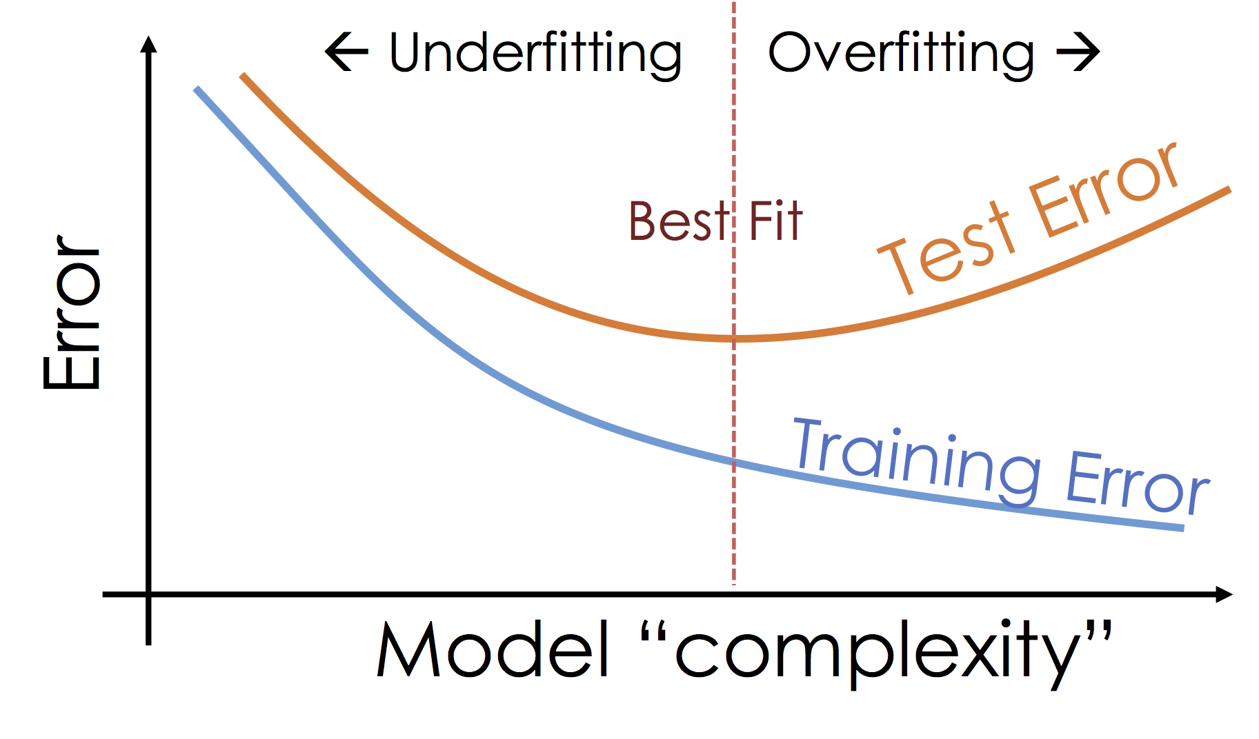
What's happening: Over-fitting

As we increase the expressiveness of our model we begin to over-fit to the variability in our training data. That is we are learning patterns that do not generalize beyond our training dataset

Over-fitting is a key challenge in machine learning and statistical inference. At it's core is a fundamental trade-off between bias and variance: the desire to explain the training data and yet be robust to variation in the training data.

We will study the bias-variance trade-off in feuture lectures but for now we will focus on the trade-off between under fitting and over fitting: