DataTables, Indexes, Pandas, and Seaborn¶

Some useful (free) resources¶

Introductory:

Getting started with Python for research, a gentle introduction to Python in data-intensive research.
A Whirlwind Tour of Python, by Jake VanderPlas, another quick Python intro (with notebooks).

Core Pandas/Data Science books:

The Python Data Science Handbook, by Jake VanderPlas.
Python for Data Analysis, 2nd Edition, by Wes McKinney, creator of Pandas. Companion Notebooks
Effective Pandas, a book by Tom Augspurger, core Pandas developer.

Complementary resources:

An introduction to "Data Science", a collection of Notebooks by BIDS' Stéfan Van der Walt.
Effective Computation in Physics, by Kathryn D. Huff; Anthony Scopatz. Notebooks to accompany the book. Don't be fooled by the title, it's a great book on modern computational practices with very little that's physics-specific.

OK, let's load and configure some of our core libraries (as an aside, you can find a nice visual gallery of available matplotlib sytles here).

%matplotlib inline
import matplotlib.pyplot as plt
import seaborn as sns
import numpy as np
import pandas as pd

plt.style.use('fivethirtyeight')
sns.set_context("notebook")

Getting the Data¶

https://www.ssa.gov/OACT/babynames/index.html

https://www.ssa.gov/data

As we saw before, we can download data from the internet with Python, and do so only if needed:

import requests
from pathlib import Path

namesbystate_path = Path('namesbystate.zip')
data_url = 'https://www.ssa.gov/oact/babynames/state/namesbystate.zip'

if not namesbystate_path.exists():
    print('Downloading...', end=' ')
    resp = requests.get(data_url)
    with namesbystate_path.open('wb') as f:
        f.write(resp.content)
    print('Done!')

Let's use Python to understand how this data is laid out:

import zipfile
zf = zipfile.ZipFile(namesbystate_path, 'r')
print([f.filename for f in zf.filelist])

['DC.TXT', 'DE.TXT', 'FL.TXT', 'GA.TXT', 'HI.TXT', 'IA.TXT', 'ID.TXT', 'IL.TXT', 'IN.TXT', 'KS.TXT', 'KY.TXT', 'LA.TXT', 'MA.TXT', 'MD.TXT', 'ME.TXT', 'MI.TXT', 'MN.TXT', 'MO.TXT', 'MS.TXT', 'MT.TXT', 'NC.TXT', 'ND.TXT', 'NE.TXT', 'NH.TXT', 'NJ.TXT', 'NM.TXT', 'NV.TXT', 'NY.TXT', 'OH.TXT', 'OK.TXT', 'OR.TXT', 'PA.TXT', 'RI.TXT', 'SC.TXT', 'SD.TXT', 'TN.TXT', 'TX.TXT', 'UT.TXT', 'VA.TXT', 'VT.TXT', 'WA.TXT', 'WI.TXT', 'WV.TXT', 'WY.TXT', 'AK.TXT', 'AL.TXT', 'AR.TXT', 'AZ.TXT', 'CA.TXT', 'CO.TXT', 'CT.TXT', 'StateReadMe.pdf']

We can pull the PDF readme to view it, but let's operate with the rest of the data in its compressed state:

zf.extract('StateReadMe.pdf')

'/Users/fperez/teach/ds100/sp18-dev/lectures/lec03/StateReadMe.pdf'

Let's have a look at the California data, it should give us an idea about the structure of the whole thing:

ca_name = 'CA.TXT'
with zf.open(ca_name) as f:
    for i in range(10):
        print(f.readline().rstrip().decode())

CA,F,1910,Mary,295
CA,F,1910,Helen,239
CA,F,1910,Dorothy,220
CA,F,1910,Margaret,163
CA,F,1910,Frances,134
CA,F,1910,Ruth,128
CA,F,1910,Evelyn,126
CA,F,1910,Alice,118
CA,F,1910,Virginia,101
CA,F,1910,Elizabeth,93

This is equivalent (on macOS or Linux) to extracting the full CA.TXT file to disk and then using the head command (if you're on Windows, don't try to run the cell below):

zf.extract(ca_name)
!head {ca_name}

!echo {ca_name}

CA.TXT

A couple of practical comments:

The above is using special tricks in IPython that let you call operating system commands via !cmd, and that expand Python variables in such commands with the {var} syntax. You can find more about IPython's special tricks in this tutorial.
head doesn't work on Windows, though there are equivalent Windows commands. But by using Python code, even if it's a little bit more verbose, we have a 100% portable solution.
If the CA.TXT file was huge, it would be wasteful to write it all to disk only to look at the start of the file.

The last point is an important, and general theme of this course: we need to learn how to operate with data only on an as-needed basis, because there are many situations in the real world where we can't afford to brute-force 'download all the things'.

Let's remove the CA.TXT file to make sure we keep working with our compressed data, as if we couldn't extract it:

import os; os.unlink(ca_name)

Question 1: What was the most popular name in CA last year?¶

import pandas as pd

field_names = ['State', 'Sex', 'Year', 'Name', 'Count']
with zf.open(ca_name) as fh:
    ca = pd.read_csv(fh, header=None, names=field_names)
ca.head()

Slicing¶

A Pandas DataFrame is, by default, indexed by column name:

ca['Count'].head()

0    295
1    239
2    220
3    163
4    134
Name: Count, dtype: int64

ca[0:3]

#ca[0]

ca.iloc[:3, -2:]

ca.loc[0:3, 'State']

0    CA
1    CA
2    CA
3    CA
Name: State, dtype: object

ca['Name'].head()

0        Mary
1       Helen
2     Dorothy
3    Margaret
4     Frances
Name: Name, dtype: object

ca[['Name']].head()

For more on loc and iloc, see the pandas documentation.

Now, what is the leftmost column?

emails = ca.head()
emails.index = ['a@gmail.com', 'b@gmail.com', 'c@gmail.com', 'd@gmail.com', 'e@gmail.com']
emails

emails.loc['b@gmail.com':'d@gmail.com', 'Year':'Name']

emails.iloc[0:3]

ca.head()

(ca['Year'] == 2016).head()

0    False
1    False
2    False
3    False
4    False
Name: Year, dtype: bool

ca[ca['Year'] == 2016].tail()

Sorting¶

ca_sorted = ca[ca['Year'] == 2016]
ca_sorted.sort_values('Count', ascending=False).tail(10)

Recap: anatomy of a DataFrame¶

Let's look again at the data we have for California:

ca.head()

We can get a sense for the shape of our data:

ca.shape

(367931, 5)

ca.size  # rows x columns

1839655

Pandas will give us a summary overview of the numerical data in the DataFrame:

ca.describe()

And let's look at the structure of the DataFrame:

ca.index

RangeIndex(start=0, stop=367931, step=1)

emails

emails.index

Index(['a@gmail.com', 'b@gmail.com', 'c@gmail.com', 'd@gmail.com',
       'e@gmail.com'],
      dtype='object')

emails.index.name = 'Email'
emails

The columns can also be named, since the .columns attribute is an Index too:

emails.columns

Index(['State', 'Sex', 'Year', 'Name', 'Count'], dtype='object')

emails.columns.name = 'Fields'
emails

Note that it's possible to have an index with integers that do not correspond to the default [0, 1, 2, ...] positional order:

numbers = emails.copy()
numbers.index = [5,4,3,2,1]
numbers.index.name = 'order'
numbers.columns.name = None  # letremove name for column index for clarity
numbers

Now, the number 1 can be used to access the positionally second row, with iloc:

numbers.iloc[1]

State       CA
Sex          F
Year      1910
Name     Helen
Count      239
Name: 4, dtype: object

Or the row labeled 1, which in this case happens to be the last one:

numbers.loc[1]

State         CA
Sex            F
Year        1910
Name     Frances
Count        134
Name: 1, dtype: object

Integer/positional with iloc vs labeled with loc can be used also for multiple rows/columns:

numbers.iloc[:3, -2:]

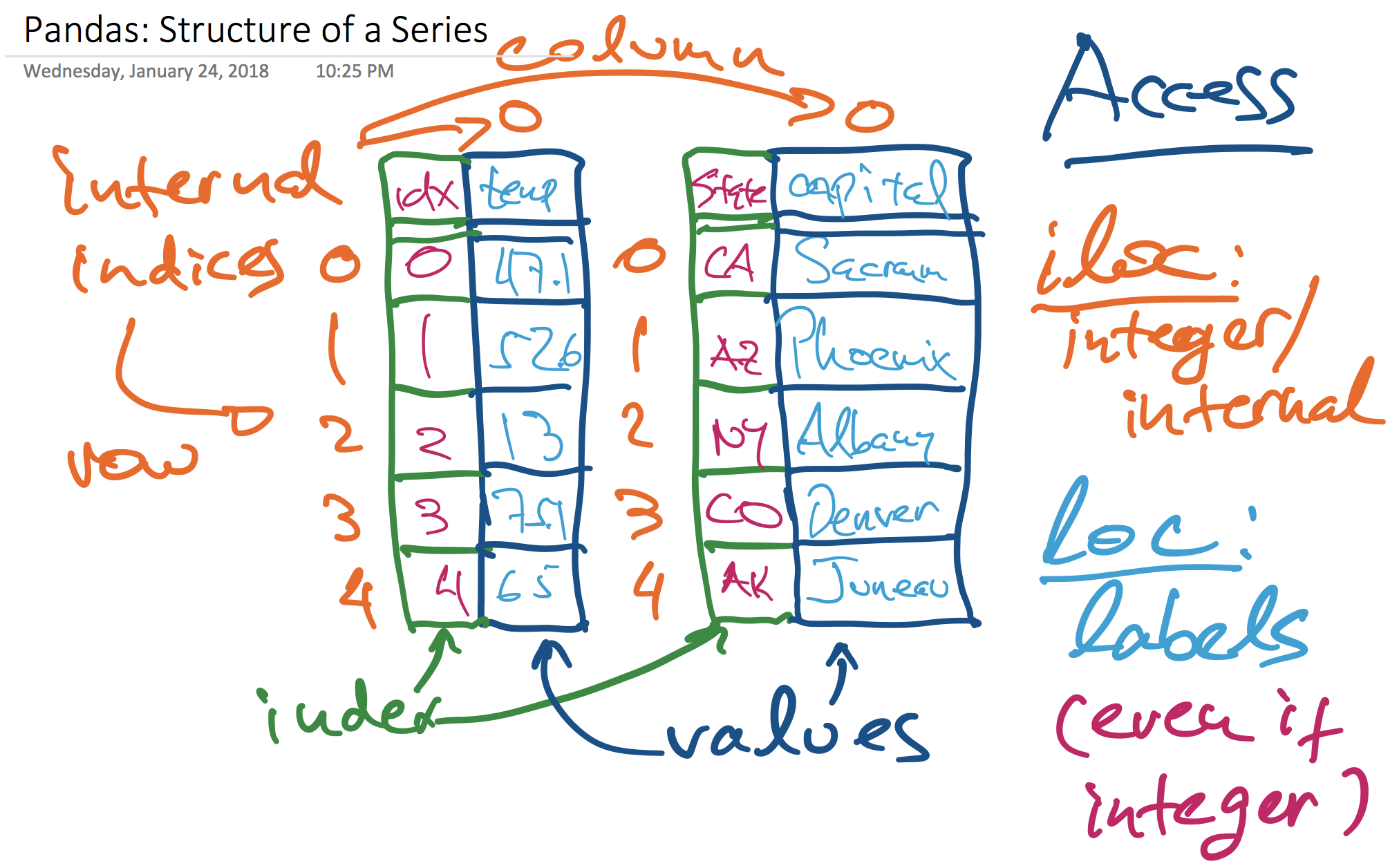
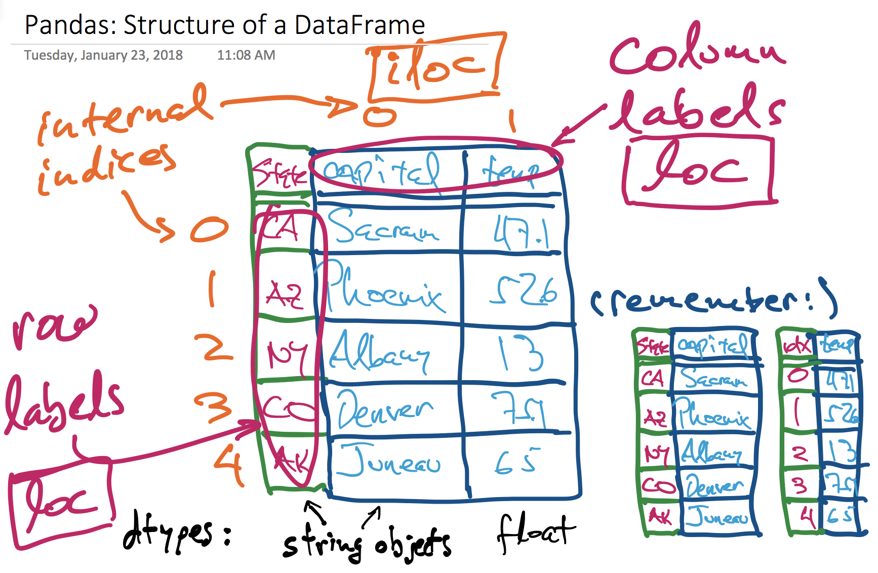
These two diagrams illustrate the various pieces that compose a Pandas Series:

and a DataFrame, which is a set of Series that share a common index:

Question 2: Most popular names in all states for each year?¶

Put all DFs together¶

Again, we'll work off our in-memory, compressed zip archive and pull the data out of it into Pandas DataFrames without ever putting it all on disk. We can see how large the compressed and uncompressed data is:

sum(f.file_size for f in zf.filelist)/1_000_000

120.463088

sum(f.compress_size for f in zf.filelist)/1_000_000

24.900652

__/_  # divide the next-previous result by the previous one

4.837748344902776

First, notice that the in-memory compressed archive is not alphabetically sorted:

zf.filelist[:5]

[<ZipInfo filename='DC.TXT' compress_type=deflate external_attr=0x20 file_size=1120459 compress_size=225154>,
 <ZipInfo filename='DE.TXT' compress_type=deflate external_attr=0x20 file_size=642699 compress_size=127631>,
 <ZipInfo filename='FL.TXT' compress_type=deflate external_attr=0x20 file_size=4057116 compress_size=848854>,
 <ZipInfo filename='GA.TXT' compress_type=deflate external_attr=0x20 file_size=3616566 compress_size=742801>,
 <ZipInfo filename='HI.TXT' compress_type=deflate external_attr=0x20 file_size=1086102 compress_size=216102>]

But we can pull them out in alphabetical order with the Python sorted function, sorting by filename:

%%time
states = []

for f in sorted(zf.filelist, key=lambda x:x.filename):
    if not f.filename.endswith('.TXT'):
        continue
    with zf.open(f) as fh:
        states.append(pd.read_csv(fh, header=None, names=field_names))

CPU times: user 2.42 s, sys: 475 ms, total: 2.9 s
Wall time: 2.92 s

Now, we create a single DataFrame by concatenating these into one:

baby_names = pd.concat(states).reset_index(drop=True)
baby_names.head()

baby_names.shape

(5838786, 5)

Group by state and year¶

baby_names[
    (baby_names['State'] == 'CA')
    & (baby_names['Year'] == 1995)
    & (baby_names['Sex'] == 'M')
].head()

# Now I could write 3 nested for loops...

%%time
baby_names.groupby('State').size().head()

CPU times: user 162 ms, sys: 84.6 ms, total: 246 ms
Wall time: 243 ms

State
AK     27624
AL    130297
AR     98853
AZ    110866
CA    367931
dtype: int64

state_counts = baby_names.loc[:, ('State', 'Count')]
state_counts.head()

sg = state_counts.groupby('State')
sg

<pandas.core.groupby.DataFrameGroupBy object at 0x10c913128>

Pause: what is a `DataFrameGroupBy` object?¶

See companion notebook, and come back...

You're back. Let's continue with our question¶

(Finding the most popular baby names for all states and years).

state_counts.groupby('State').sum().head()

state_counts.group('State', np.sum)

import numpy as np
state_counts.groupby('State').agg(np.sum).head()

Using a custom function to aggregate.

Equivalent to this code from Data 8:

state_and_groups.group('State', np.sum)

Grouping by multiple columns¶

baby_names.groupby(['State', 'Year']).size().head(3)

State  Year
AK     1910    16
       1911    11
       1912    20
dtype: int64

baby_names.groupby(['State', 'Year']).sum().head(3)

ak1910 = baby_names.query("State=='AK' and Year==1910")
print(ak1910.shape)
ak1910

(16, 5)

baby_names.groupby(['State', 'Year', 'Sex']).sum().head()

%%time
def first(series):
    '''Returns the first value in the series.'''
    return series.iloc[0]

most_popular_names = (
    baby_names
    .groupby(['State', 'Year', 'Sex'])
    .agg(first)
)
most_popular_names.head()

CPU times: user 913 ms, sys: 302 ms, total: 1.21 s
Wall time: 1.22 s

This creates a multilevel index. It is quite complex, but just know that you can still slice:

most_popular_names[most_popular_names['Name'] == 'Samuel']

And you can use .loc as so:

most_popular_names.loc['CA', 1997, 'M']

Name     Daniel
Count      4452
Name: (CA, 1997, M), dtype: object

most_popular_names.loc['CA', 1995:2000, 'M']

Question 3: Can I deduce birth sex from the last letter of a person’s name?¶

Compute last letter of each name¶

baby_names.head()

baby_names['Name'].apply(len).head()

0    4
1    5
2    4
3    8
4    5
Name: Name, dtype: int64

baby_names['Name'].str.len().head()

0    4
1    5
2    4
3    8
4    5
Name: Name, dtype: int64

baby_names['Name'].str[-1].head()

0    y
1    e
2    a
3    t
4    n
Name: Name, dtype: object

To add column to dataframe:

baby_names['Last letter'] = baby_names['Name'].str[-1]
baby_names.head()

Group by last letter and sex¶

letter_counts = (baby_names
                 .loc[:, ('Sex', 'Count', 'Last letter')]
                 .groupby(['Last letter', 'Sex'])
                 .sum())
letter_counts.head()

Visualize our result¶

Use .plot to get some basic plotting functionality:

# Why is this not good?
letter_counts.plot.barh(figsize=(15, 15));

Reading the docs shows me that pandas will make one set of bars for each column in my table. How do I move each sex into its own column? I have to use pivot:

# For comparison, the group above:
# letter_counts = (baby_names
#                  .loc[:, ('Sex', 'Count', 'Last letter')]
#                  .groupby(['Last letter', 'Sex'])
#                  .sum())

last_letter_pivot = baby_names.pivot_table(
    index='Last letter', # the rows (turned into index)
    columns='Sex', # the column values
    values='Count', # the field(s) to processed in each group
    aggfunc=sum, # group operation
)
last_letter_pivot.head()

Slides: GroupBy/Pivot comparison slides and Quiz¶

At this point, I highly recommend this very nice tutorial on Pivot Tables.

last_letter_pivot.plot.barh(figsize=(10, 10));

Why is this still not ideal?

Plotting raw counts
Not sorted by any order

totals = last_letter_pivot['F'] + last_letter_pivot['M']

last_letter_props = pd.DataFrame({
    'F': last_letter_pivot['F'] / totals,
    'M': last_letter_pivot['M'] / totals,
}).sort_values('M')
last_letter_props.head()

last_letter_props.plot.barh(figsize=(10, 10));

What do you notice?

Seaborn¶

Let's use a subset of our dataset for now:

ca_and_ny = baby_names[
    (baby_names['Year'] == 2016)
    & (baby_names['State'].isin(['CA', 'NY']))
].reset_index(drop=True)
ca_and_ny.head()

Note that the same thing can be computed as a query:

baby_names.query("Year==2016 and State in ['CA', 'NY']").reset_index(drop=True).head()

We actually don't need to do any pivoting / grouping for seaborn!

sns.barplot(x='Sex', y='Count', data=ca_and_ny);

Note the automatic confidence interval generation. Many seaborn functions have these nifty statistical features.

(It actually isn't useful for our case since we have a census. It also makes seaborn functions run slower since they use bootstrap to generate the CI, so sometimes you want to turn it off.)

sns.barplot(x='Sex', y='Count', data=ca_and_ny, estimator=sum);

sns.barplot(x='State', y='Count', hue='Sex', data=ca_and_ny, ci=None, estimator=sum);

Going to work with tips data just to demonstrate:

tips = sns.load_dataset("tips")
tips.head()

sns.distplot(tips['total_bill']);

sns.lmplot(x="total_bill", y="tip", data=tips);

sns.lmplot(x="total_bill", y="tip", hue='smoker', data=tips);

sns.lmplot(x="total_bill", y="tip", col="smoker", data=tips);

	Year	Count
count	367931.000000	367931.000000
mean	1982.117169	81.850034
std	25.928678	303.826855
min	1910.000000	5.000000
25%	1966.000000	7.000000
50%	1988.000000	13.000000
75%	2003.000000	39.000000
max	2016.000000	8263.000000

		Count
Last letter	Sex
a	F	49128453
a	M	1585024
b	F	9666
b	M	1369244
c	F	18211

Sex	F	M
Last letter
a	49128453	1585024
b	9666	1369244
c	18211	1565621
d	564804	15423771
e	31212081	12778932

	F	M
Last letter
a	0.968746	0.031254
i	0.830335	0.169665
e	0.709510	0.290490
z	0.645210	0.354790
y	0.571341	0.428659

	total_bill	tip	sex	smoker	day	time	size
0	16.99	1.01	Female	No	Sun	Dinner	2
1	10.34	1.66	Male	No	Sun	Dinner	3
2	21.01	3.50	Male	No	Sun	Dinner	3
3	23.68	3.31	Male	No	Sun	Dinner	2
4	24.59	3.61	Female	No	Sun	Dinner	4

	State	Sex	Year	Name	Count
0	CA	F	1910	Mary	295
1	CA	F	1910	Helen	239
2	CA	F	1910	Dorothy	220
3	CA	F	1910	Margaret	163
4	CA	F	1910	Frances	134

	State	Sex	Year	Name	Count
a@gmail.com	CA	F	1910	Mary	295
b@gmail.com	CA	F	1910	Helen	239
c@gmail.com	CA	F	1910	Dorothy	220
d@gmail.com	CA	F	1910	Margaret	163
e@gmail.com	CA	F	1910	Frances	134

	State	Sex	Year	Name	Count
367926	CA	M	2016	Zekiel	5
367927	CA	M	2016	Ziyad	5
367928	CA	M	2016	Zorawar	5
367929	CA	M	2016	Zyan	5
367930	CA	M	2016	Zyir	5

	State	Sex	Year	Name	Count
217131	CA	F	2016	Maleena	5
217132	CA	F	2016	Maleny	5
217133	CA	F	2016	Maleya	5
217134	CA	F	2016	Mali	5
217135	CA	F	2016	Malika	5
217136	CA	F	2016	Manreet	5
217137	CA	F	2016	Manuela	5
217138	CA	F	2016	Marilee	5
217139	CA	F	2016	Marya	5
367930	CA	M	2016	Zyir	5

	State	Sex	Year	Name	Count
Email
a@gmail.com	CA	F	1910	Mary	295
b@gmail.com	CA	F	1910	Helen	239
c@gmail.com	CA	F	1910	Dorothy	220
d@gmail.com	CA	F	1910	Margaret	163
e@gmail.com	CA	F	1910	Frances	134

	State	Sex	Year	Name	Count
order
5	CA	F	1910	Mary	295
4	CA	F	1910	Helen	239
3	CA	F	1910	Dorothy	220
2	CA	F	1910	Margaret	163
1	CA	F	1910	Frances	134

	State	Sex	Year	Name	Count
675533	CA	M	1995	Daniel	5003
675534	CA	M	1995	Michael	4783
675535	CA	M	1995	Jose	4572
675536	CA	M	1995	Christopher	4096
675537	CA	M	1995	David	4029

			Name	Count
State	Year	Sex
CA	1995	M	Daniel	5003
	1996	M	Daniel	4705
	1997	M	Daniel	4452
	1998	M	Daniel	4317
	1999	M	Daniel	4352
	2000	M	Daniel	4339

	State	Sex	Year	Name	Count	Last letter
0	CA	F	2016	Mia	2785	a
1	CA	F	2016	Sophia	2747	a
2	CA	F	2016	Emma	2592	a
3	CA	F	2016	Olivia	2533	a
4	CA	F	2016	Isabella	2350	a

	Count
State
AK	424852
AL	5773719
AR	3408590
AZ	3532872
CA	30115165

	Count
State
AK	424852
AL	5773719
AR	3408590
AZ	3532872
CA	30115165