Lecture 3 – Data 100, Fall 2024
Data 100, Fall 2024
A demonstration of advanced pandas syntax to accompany Lecture 3.
import numpy as np
import pandas as pd
# Loading the elections DataFrame
elections = pd.read_csv("data/elections.csv")

elections.head()
| Year | Candidate | Party | Popular vote | Result | % | |
|---|---|---|---|---|---|---|
| 0 | 1824 | Andrew Jackson | Democratic-Republican | 151271 | loss | 57.210122 |
| 1 | 1824 | John Quincy Adams | Democratic-Republican | 113142 | win | 42.789878 |
| 2 | 1828 | Andrew Jackson | Democratic | 642806 | win | 56.203927 |
| 3 | 1828 | John Quincy Adams | National Republican | 500897 | loss | 43.796073 |
| 4 | 1832 | Andrew Jackson | Democratic | 702735 | win | 54.574789 |
Integer-Based Extraction Using iloc
iloc selects items by row and column integer position.
Arguments to .iloc can be:
- A list.
- A slice (syntax is exclusive of the right hand side of the slice).
- A single value.
# Select the rows at positions 1, 2, and 3.
# Select the columns at positions 0, 1, and 2.
# Remember that Python indexing begins at position 0!
elections.iloc[[1, 2, 3], [0, 1, 2]]
| Year | Candidate | Party | |
|---|---|---|---|
| 1 | 1824 | John Quincy Adams | Democratic-Republican |
| 2 | 1828 | Andrew Jackson | Democratic |
| 3 | 1828 | John Quincy Adams | National Republican |
# Index-based extraction using a list of rows and a slice of
# column integer positions
elections.iloc[[1, 2, 3], 0:3]
| Year | Candidate | Party | |
|---|---|---|---|
| 1 | 1824 | John Quincy Adams | Democratic-Republican |
| 2 | 1828 | Andrew Jackson | Democratic |
| 3 | 1828 | John Quincy Adams | National Republican |
# Selecting all rows using a colon
elections.iloc[:, 0:3]
| Year | Candidate | Party | |
|---|---|---|---|
| 0 | 1824 | Andrew Jackson | Democratic-Republican |
| 1 | 1824 | John Quincy Adams | Democratic-Republican |
| 2 | 1828 | Andrew Jackson | Democratic |
| 3 | 1828 | John Quincy Adams | National Republican |
| 4 | 1832 | Andrew Jackson | Democratic |
| ... | ... | ... | ... |
| 177 | 2016 | Jill Stein | Green |
| 178 | 2020 | Joseph Biden | Democratic |
| 179 | 2020 | Donald Trump | Republican |
| 180 | 2020 | Jo Jorgensen | Libertarian |
| 181 | 2020 | Howard Hawkins | Green |
182 rows × 3 columns
# Extracting data from one column
elections.iloc[[1, 2, 3], 1]
1    John Quincy Adams
2       Andrew Jackson
3    John Quincy Adams
Name: Candidate, dtype: object
# Extracting the value at row 0 and the second column
elections.iloc[0,1]
'Andrew Jackson'
Context-dependent Extraction using []
We could technically do anything we want using loc or iloc. However, in practice, the [] operator is often used instead to yield more concise code.
[] is a bit trickier to understand than loc or iloc, but it achieves essentially the same functionality. The difference is that [] is context-dependent.
[] only takes one argument, which may be:
- A slice of row integers.
- A list of column labels.
- A single column label.
If we provide a slice of row numbers, we get the numbered rows.
elections[3:7]
| Year | Candidate | Party | Popular vote | Result | % | |
|---|---|---|---|---|---|---|
| 3 | 1828 | John Quincy Adams | National Republican | 500897 | loss | 43.796073 |
| 4 | 1832 | Andrew Jackson | Democratic | 702735 | win | 54.574789 |
| 5 | 1832 | Henry Clay | National Republican | 484205 | loss | 37.603628 |
| 6 | 1832 | William Wirt | Anti-Masonic | 100715 | loss | 7.821583 |
If we provide a list of column names, we get the listed columns.
elections[["Year", "Candidate", "Result"]]
| Year | Candidate | Result | |
|---|---|---|---|
| 0 | 1824 | Andrew Jackson | loss |
| 1 | 1824 | John Quincy Adams | win |
| 2 | 1828 | Andrew Jackson | win |
| 3 | 1828 | John Quincy Adams | loss |
| 4 | 1832 | Andrew Jackson | win |
| ... | ... | ... | ... |
| 177 | 2016 | Jill Stein | loss |
| 178 | 2020 | Joseph Biden | win |
| 179 | 2020 | Donald Trump | loss |
| 180 | 2020 | Jo Jorgensen | loss |
| 181 | 2020 | Howard Hawkins | loss |
182 rows × 3 columns
And if we provide a single column name we get back just that column, stored as a Series.
elections["Candidate"]
0         Andrew Jackson
1      John Quincy Adams
2         Andrew Jackson
3      John Quincy Adams
4         Andrew Jackson
             ...
177           Jill Stein
178         Joseph Biden
179         Donald Trump
180         Jo Jorgensen
181       Howard Hawkins
Name: Candidate, Length: 182, dtype: object
Slido Exercise
weird = pd.DataFrame({"a":["one fish", "two fish"],
                      "b":["red fish", "blue fish"]})
weird
| a | b | |
|---|---|---|
| 0 | one fish | red fish |
| 1 | two fish | blue fish |
weird.iloc[1, 1]
'blue fish'
# weird.loc[1, 1]
weird.iloc[1, :]
a     two fish
b    blue fish
Name: 1, dtype: object
weird.loc[1, 'b']
'blue fish'
weird.iloc[1, 0]
'two fish'
Dataset: California baby names
In today's lecture, we'll work with the babynames dataset, which contains information about the names of infants born in California.
The cell below pulls census data from a government website and then loads it into a usable form. The code shown here is outside of the scope of Data 100, but you're encouraged to dig into it if you are interested!
import urllib.request
import os.path
import zipfile

data_url = "https://www.ssa.gov/oact/babynames/state/namesbystate.zip"
local_filename = "data/babynamesbystate.zip"
if not os.path.exists(local_filename): # If the data exists don't download again
    with urllib.request.urlopen(data_url) as resp, open(local_filename, 'wb') as f:
        f.write(resp.read())

zf = zipfile.ZipFile(local_filename, 'r')

ca_name = 'STATE.CA.TXT'
field_names = ['State', 'Sex', 'Year', 'Name', 'Count']
with zf.open(ca_name) as fh:
    babynames = pd.read_csv(fh, header=None, names=field_names)

babynames.head()
| State | Sex | Year | Name | Count | |
|---|---|---|---|---|---|
| 0 | CA | F | 1910 | Mary | 295 |
| 1 | CA | F | 1910 | Helen | 239 |
| 2 | CA | F | 1910 | Dorothy | 220 |
| 3 | CA | F | 1910 | Margaret | 163 |
| 4 | CA | F | 1910 | Frances | 134 |
Conditional Selection
# Ask yourself: Why is :9 is the correct slice to select the first 10 rows?
babynames_first_10_rows = babynames.loc[:9, :]

babynames_first_10_rows
| State | Sex | Year | Name | Count | |
|---|---|---|---|---|---|
| 0 | CA | F | 1910 | Mary | 295 |
| 1 | CA | F | 1910 | Helen | 239 |
| 2 | CA | F | 1910 | Dorothy | 220 |
| 3 | CA | F | 1910 | Margaret | 163 |
| 4 | CA | F | 1910 | Frances | 134 |
| 5 | CA | F | 1910 | Ruth | 128 |
| 6 | CA | F | 1910 | Evelyn | 126 |
| 7 | CA | F | 1910 | Alice | 118 |
| 8 | CA | F | 1910 | Virginia | 101 |
| 9 | CA | F | 1910 | Elizabeth | 93 |
By passing in a sequence (list, array, or Series) of boolean values, we can extract a subset of the rows in a DataFrame. We will keep only the rows that correspond to a boolean value of True.
# Notice how we have exactly 10 elements in our boolean array argument.
babynames_first_10_rows[[True, False, True, False, True, False, True, False, True, False]]
| State | Sex | Year | Name | Count | |
|---|---|---|---|---|---|
| 0 | CA | F | 1910 | Mary | 295 |
| 2 | CA | F | 1910 | Dorothy | 220 |
| 4 | CA | F | 1910 | Frances | 134 |
| 6 | CA | F | 1910 | Evelyn | 126 |
| 8 | CA | F | 1910 | Virginia | 101 |
# Or using .loc to filter a DataFrame by a Boolean array argument.
babynames_first_10_rows.loc[[True, False, True, False, True, False, True, False, True, False], :]
| State | Sex | Year | Name | Count | |
|---|---|---|---|---|---|
| 0 | CA | F | 1910 | Mary | 295 |
| 2 | CA | F | 1910 | Dorothy | 220 |
| 4 | CA | F | 1910 | Frances | 134 |
| 6 | CA | F | 1910 | Evelyn | 126 |
| 8 | CA | F | 1910 | Virginia | 101 |
Oftentimes, we'll use boolean selection to check for entries in a DataFrame that meet a particular condition.
# First, use a logical condition to generate a boolean Series
logical_operator = (babynames["Sex"] == "F")
logical_operator
0          True
1          True
2          True
3          True
4          True
          ...
407423    False
407424    False
407425    False
407426    False
407427    False
Name: Sex, Length: 407428, dtype: bool
# Then, use this boolean Series to filter the DataFrame
babynames[logical_operator]
| State | Sex | Year | Name | Count | |
|---|---|---|---|---|---|
| 0 | CA | F | 1910 | Mary | 295 |
| 1 | CA | F | 1910 | Helen | 239 |
| 2 | CA | F | 1910 | Dorothy | 220 |
| 3 | CA | F | 1910 | Margaret | 163 |
| 4 | CA | F | 1910 | Frances | 134 |
| ... | ... | ... | ... | ... | ... |
| 239532 | CA | F | 2022 | Zemira | 5 |
| 239533 | CA | F | 2022 | Ziggy | 5 |
| 239534 | CA | F | 2022 | Zimal | 5 |
| 239535 | CA | F | 2022 | Zosia | 5 |
| 239536 | CA | F | 2022 | Zulay | 5 |
239537 rows × 5 columns
Boolean selection also works with loc!
# Notice that we did not have to specify columns to select
# If no columns are referenced, pandas will automatically select all columns
babynames.loc[babynames["Sex"] == "F"]
| State | Sex | Year | Name | Count | |
|---|---|---|---|---|---|
| 0 | CA | F | 1910 | Mary | 295 |
| 1 | CA | F | 1910 | Helen | 239 |
| 2 | CA | F | 1910 | Dorothy | 220 |
| 3 | CA | F | 1910 | Margaret | 163 |
| 4 | CA | F | 1910 | Frances | 134 |
| ... | ... | ... | ... | ... | ... |
| 239532 | CA | F | 2022 | Zemira | 5 |
| 239533 | CA | F | 2022 | Ziggy | 5 |
| 239534 | CA | F | 2022 | Zimal | 5 |
| 239535 | CA | F | 2022 | Zosia | 5 |
| 239536 | CA | F | 2022 | Zulay | 5 |
239537 rows × 5 columns
To filter on multiple conditions, we combine boolean operators using bitwise comparisons.
| Symbol | Usage | Meaning |
|---|---|---|
| ~ | ~p | Returns negation of p |
| | | p | q | p OR q |
| & | p & q | p AND q |
| ^ | p ^ q | p XOR q (exclusive or) |
babynames[(babynames["Sex"] == "F") & (babynames["Year"] < 2000)]
| State | Sex | Year | Name | Count | |
|---|---|---|---|---|---|
| 0 | CA | F | 1910 | Mary | 295 |
| 1 | CA | F | 1910 | Helen | 239 |
| 2 | CA | F | 1910 | Dorothy | 220 |
| 3 | CA | F | 1910 | Margaret | 163 |
| 4 | CA | F | 1910 | Frances | 134 |
| ... | ... | ... | ... | ... | ... |
| 149050 | CA | F | 1999 | Zareen | 5 |
| 149051 | CA | F | 1999 | Zeinab | 5 |
| 149052 | CA | F | 1999 | Zhane | 5 |
| 149053 | CA | F | 1999 | Zoha | 5 |
| 149054 | CA | F | 1999 | Zoila | 5 |
149055 rows × 5 columns
babynames[(babynames["Sex"] == "F") | (babynames["Year"] < 2000)]
| State | Sex | Year | Name | Count | |
|---|---|---|---|---|---|
| 0 | CA | F | 1910 | Mary | 295 |
| 1 | CA | F | 1910 | Helen | 239 |
| 2 | CA | F | 1910 | Dorothy | 220 |
| 3 | CA | F | 1910 | Margaret | 163 |
| 4 | CA | F | 1910 | Frances | 134 |
| ... | ... | ... | ... | ... | ... |
| 342435 | CA | M | 1999 | Yuuki | 5 |
| 342436 | CA | M | 1999 | Zakariya | 5 |
| 342437 | CA | M | 1999 | Zavier | 5 |
| 342438 | CA | M | 1999 | Zayn | 5 |
| 342439 | CA | M | 1999 | Zayne | 5 |
342440 rows × 5 columns
babynames.iloc[[0, 233, 484], [3, 4]]
| Name | Count | |
|---|---|---|
| 0 | Mary | 295 |
| 233 | Mary | 390 |
| 484 | Mary | 534 |
babynames.loc[[0, 233, 484]]
| State | Sex | Year | Name | Count | |
|---|---|---|---|---|---|
| 0 | CA | F | 1910 | Mary | 295 |
| 233 | CA | F | 1911 | Mary | 390 |
| 484 | CA | F | 1912 | Mary | 534 |
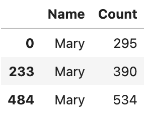
babynames.loc[babynames["Count"] > 250, ["Name", "Count"]].head(3)
| Name | Count | |
|---|---|---|
| 0 | Mary | 295 |
| 233 | Mary | 390 |
| 484 | Mary | 534 |
babynames.loc[babynames["Count"] > 250, ["Name", "Count"]].iloc[0:2, :]
| Name | Count | |
|---|---|---|
| 0 | Mary | 295 |
| 233 | Mary | 390 |
# Note: The parentheses surrounding the code make it possible to
# break the code into multiple lines for readability

(
    babynames[(babynames["Name"] == "Bella") |
              (babynames["Name"] == "Alex") |
              (babynames["Name"] == "Narges") |
              (babynames["Name"] == "Lisa")]
)
| State | Sex | Year | Name | Count | |
|---|---|---|---|---|---|
| 6289 | CA | F | 1923 | Bella | 5 |
| 7512 | CA | F | 1925 | Bella | 8 |
| 12368 | CA | F | 1932 | Lisa | 5 |
| 14741 | CA | F | 1936 | Lisa | 8 |
| 17084 | CA | F | 1939 | Lisa | 5 |
| ... | ... | ... | ... | ... | ... |
| 393248 | CA | M | 2018 | Alex | 495 |
| 396111 | CA | M | 2019 | Alex | 438 |
| 398983 | CA | M | 2020 | Alex | 379 |
| 401788 | CA | M | 2021 | Alex | 333 |
| 404663 | CA | M | 2022 | Alex | 344 |
317 rows × 5 columns
# A more concise method to achieve the above: .isin
names = ["Bella", "Alex", "Narges", "Lisa"]
display(babynames["Name"].isin(names))
display(babynames[babynames["Name"].isin(names)])
0         False
1         False
2         False
3         False
4         False
          ...
407423    False
407424    False
407425    False
407426    False
407427    False
Name: Name, Length: 407428, dtype: bool
| State | Sex | Year | Name | Count | |
|---|---|---|---|---|---|
| 6289 | CA | F | 1923 | Bella | 5 |
| 7512 | CA | F | 1925 | Bella | 8 |
| 12368 | CA | F | 1932 | Lisa | 5 |
| 14741 | CA | F | 1936 | Lisa | 8 |
| 17084 | CA | F | 1939 | Lisa | 5 |
| ... | ... | ... | ... | ... | ... |
| 393248 | CA | M | 2018 | Alex | 495 |
| 396111 | CA | M | 2019 | Alex | 438 |
| 398983 | CA | M | 2020 | Alex | 379 |
| 401788 | CA | M | 2021 | Alex | 333 |
| 404663 | CA | M | 2022 | Alex | 344 |
317 rows × 5 columns
# What if we only want names that start with "N"?
display(babynames["Name"].str.startswith("N"))

display(babynames[babynames["Name"].str.startswith("N")])
0         False
1         False
2         False
3         False
4         False
          ...
407423    False
407424    False
407425    False
407426    False
407427    False
Name: Name, Length: 407428, dtype: bool
| State | Sex | Year | Name | Count | |
|---|---|---|---|---|---|
| 76 | CA | F | 1910 | Norma | 23 |
| 83 | CA | F | 1910 | Nellie | 20 |
| 127 | CA | F | 1910 | Nina | 11 |
| 198 | CA | F | 1910 | Nora | 6 |
| 310 | CA | F | 1911 | Nellie | 23 |
| ... | ... | ... | ... | ... | ... |
| 407319 | CA | M | 2022 | Nilan | 5 |
| 407320 | CA | M | 2022 | Niles | 5 |
| 407321 | CA | M | 2022 | Nolen | 5 |
| 407322 | CA | M | 2022 | Noriel | 5 |
| 407323 | CA | M | 2022 | Norris | 5 |
12229 rows × 5 columns
Adding, Removing, and Modifying Columns
To add a column, use [] to reference the desired new column, then assign it to a Series or array of appropriate length.
# Create a Series of the length of each name.
babyname_lengths = babynames["Name"].str.len()

# Add a column named "name_lengths" that includes the length of each name.
babynames["name_lengths"] = babyname_lengths

babynames
| State | Sex | Year | Name | Count | name_lengths | |
|---|---|---|---|---|---|---|
| 0 | CA | F | 1910 | Mary | 295 | 4 |
| 1 | CA | F | 1910 | Helen | 239 | 5 |
| 2 | CA | F | 1910 | Dorothy | 220 | 7 |
| 3 | CA | F | 1910 | Margaret | 163 | 8 |
| 4 | CA | F | 1910 | Frances | 134 | 7 |
| ... | ... | ... | ... | ... | ... | ... |
| 407423 | CA | M | 2022 | Zayvier | 5 | 7 |
| 407424 | CA | M | 2022 | Zia | 5 | 3 |
| 407425 | CA | M | 2022 | Zora | 5 | 4 |
| 407426 | CA | M | 2022 | Zuriel | 5 | 6 |
| 407427 | CA | M | 2022 | Zylo | 5 | 4 |
407428 rows × 6 columns
To modify a column, use [] to access the desired column, then re-assign it to a new array or Series.
# Modify the "name_lengths" column to be one less than its original value.
babynames["name_lengths"] = babynames["name_lengths"] - 1
babynames
| State | Sex | Year | Name | Count | name_lengths | |
|---|---|---|---|---|---|---|
| 0 | CA | F | 1910 | Mary | 295 | 3 |
| 1 | CA | F | 1910 | Helen | 239 | 4 |
| 2 | CA | F | 1910 | Dorothy | 220 | 6 |
| 3 | CA | F | 1910 | Margaret | 163 | 7 |
| 4 | CA | F | 1910 | Frances | 134 | 6 |
| ... | ... | ... | ... | ... | ... | ... |
| 407423 | CA | M | 2022 | Zayvier | 5 | 6 |
| 407424 | CA | M | 2022 | Zia | 5 | 2 |
| 407425 | CA | M | 2022 | Zora | 5 | 3 |
| 407426 | CA | M | 2022 | Zuriel | 5 | 5 |
| 407427 | CA | M | 2022 | Zylo | 5 | 3 |
407428 rows × 6 columns
Rename a column using the .rename() method.
# Rename "name_lengths" to "Length".
babynames = babynames.rename(columns={"name_lengths":"Length"})
babynames
| State | Sex | Year | Name | Count | Length | |
|---|---|---|---|---|---|---|
| 0 | CA | F | 1910 | Mary | 295 | 3 |
| 1 | CA | F | 1910 | Helen | 239 | 4 |
| 2 | CA | F | 1910 | Dorothy | 220 | 6 |
| 3 | CA | F | 1910 | Margaret | 163 | 7 |
| 4 | CA | F | 1910 | Frances | 134 | 6 |
| ... | ... | ... | ... | ... | ... | ... |
| 407423 | CA | M | 2022 | Zayvier | 5 | 6 |
| 407424 | CA | M | 2022 | Zia | 5 | 2 |
| 407425 | CA | M | 2022 | Zora | 5 | 3 |
| 407426 | CA | M | 2022 | Zuriel | 5 | 5 |
| 407427 | CA | M | 2022 | Zylo | 5 | 3 |
407428 rows × 6 columns
Remove a column using .drop().
# Remove our new "Length" column.
babynames = babynames.drop("Length", axis="columns")
babynames
| State | Sex | Year | Name | Count | |
|---|---|---|---|---|---|
| 0 | CA | F | 1910 | Mary | 295 |
| 1 | CA | F | 1910 | Helen | 239 |
| 2 | CA | F | 1910 | Dorothy | 220 |
| 3 | CA | F | 1910 | Margaret | 163 |
| 4 | CA | F | 1910 | Frances | 134 |
| ... | ... | ... | ... | ... | ... |
| 407423 | CA | M | 2022 | Zayvier | 5 |
| 407424 | CA | M | 2022 | Zia | 5 |
| 407425 | CA | M | 2022 | Zora | 5 |
| 407426 | CA | M | 2022 | Zuriel | 5 |
| 407427 | CA | M | 2022 | Zylo | 5 |
407428 rows × 5 columns
Useful Utility Functions
NumPy
The NumPy functions you encountered in Data 8 are compatible with objects in pandas.
yash_counts = babynames[babynames["Name"] == "Yash"]["Count"]
yash_counts
331824     8
334114     9
336390    11
338773    12
341387    10
343571    14
345767    24
348230    29
350889    24
353445    29
356221    25
358978    27
361831    29
364905    24
367867    23
370945    18
374055    14
376756    18
379660    18
383338     9
385903    12
388529    17
391485    16
394906    10
397874     9
400171    15
403092    13
406006    13
Name: Count, dtype: int64
# Average number of babies named Yash each year

np.mean(yash_counts)
17.142857142857142
# Max number of babies named Yash born in any single year

max(yash_counts)
29
Built-In pandas Methods
There are many, many utility functions built into pandas, far more than we can possibly cover in lecture. You are encouraged to explore all the functionality outlined in the pandas documentation.
# Returns the shape of the object in the format (num_rows, num_columns)
babynames.shape
(407428, 5)
# Returns the total number of entries in the object, equal to num_rows * num_columns
babynames.size
2037140
# What summary statistics can we describe?
babynames.describe()
| Year | Count | |
|---|---|---|
| count | 407428.000000 | 407428.000000 |
| mean | 1985.733609 | 79.543456 |
| std | 27.007660 | 293.698654 |
| min | 1910.000000 | 5.000000 |
| 25% | 1969.000000 | 7.000000 |
| 50% | 1992.000000 | 13.000000 |
| 75% | 2008.000000 | 38.000000 |
| max | 2022.000000 | 8260.000000 |
# Our statistics are slightly different when working with a Series.
babynames["Sex"].describe()
count     407428
unique         2
top            F
freq      239537
Name: Sex, dtype: object
# Randomly sample row(s) from the DataFrame.
babynames.sample()
| State | Sex | Year | Name | Count | |
|---|---|---|---|---|---|
| 154936 | CA | F | 2001 | Darya | 10 |
# Rerun this cell a few times – you'll get different results!
babynames.sample(5).iloc[:, 2:]
| Year | Name | Count | |
|---|---|---|---|
| 339370 | 1998 | Vito | 7 |
| 99351 | 1985 | Janea | 5 |
| 386376 | 2015 | Reilly | 8 |
| 15857 | 1938 | Sherry | 40 |
| 118930 | 1991 | Tatum | 8 |
# Sampling with replacement.
babynames[babynames["Year"] == 2000].sample(4, replace = True).iloc[:,2:]
| Year | Name | Count | |
|---|---|---|---|
| 344801 | 2000 | Justine | 5 |
| 151714 | 2000 | Cloey | 7 |
| 342700 | 2000 | Troy | 158 |
| 152033 | 2000 | Evelina | 6 |
# Count the number of times each unique value occurs in a Series.
babynames["Name"].value_counts()
Name
Jean         223
Francis      221
Guadalupe    218
Jessie       217
Marion       214
            ...
Renesme        1
Purity         1
Olanna         1
Nohea          1
Zayvier        1
Name: count, Length: 20437, dtype: int64
# Return an array of all unique values in the Series.
babynames["Name"].unique()
array(['Mary', 'Helen', 'Dorothy', ..., 'Zae', 'Zai', 'Zayvier'],
      dtype=object)
# Sort a Series.
babynames["Name"].sort_values()
366001      Aadan
384005      Aadan
369120      Aadan
398211    Aadarsh
370306      Aaden
           ...
220691      Zyrah
197529      Zyrah
217429      Zyrah
232167      Zyrah
404544      Zyrus
Name: Name, Length: 407428, dtype: object
# Sort a DataFrame – there are lots of Michaels in California.
babynames.sort_values(by="Count", ascending=False)
| State | Sex | Year | Name | Count | |
|---|---|---|---|---|---|
| 268041 | CA | M | 1957 | Michael | 8260 |
| 267017 | CA | M | 1956 | Michael | 8258 |
| 317387 | CA | M | 1990 | Michael | 8246 |
| 281850 | CA | M | 1969 | Michael | 8245 |
| 283146 | CA | M | 1970 | Michael | 8196 |
| ... | ... | ... | ... | ... | ... |
| 317292 | CA | M | 1989 | Olegario | 5 |
| 317291 | CA | M | 1989 | Norbert | 5 |
| 317290 | CA | M | 1989 | Niles | 5 |
| 317289 | CA | M | 1989 | Nikola | 5 |
| 407427 | CA | M | 2022 | Zylo | 5 |
407428 rows × 5 columns
# Create a Series of the length of each name.
babyname_lengths = babynames["Name"].str.len()

# Add a column named "name_lengths" that includes the length of each name.
babynames["name_lengths"] = babyname_lengths
babynames.head(5)
| State | Sex | Year | Name | Count | name_lengths | |
|---|---|---|---|---|---|---|
| 0 | CA | F | 1910 | Mary | 295 | 4 |
| 1 | CA | F | 1910 | Helen | 239 | 5 |
| 2 | CA | F | 1910 | Dorothy | 220 | 7 |
| 3 | CA | F | 1910 | Margaret | 163 | 8 |
| 4 | CA | F | 1910 | Frances | 134 | 7 |
# Sort by the temporary column.
babynames = babynames.sort_values(by="name_lengths", ascending=False)
babynames.head(5)
| State | Sex | Year | Name | Count | name_lengths | |
|---|---|---|---|---|---|---|
| 334166 | CA | M | 1996 | Franciscojavier | 8 | 15 |
| 337301 | CA | M | 1997 | Franciscojavier | 5 | 15 |
| 339472 | CA | M | 1998 | Franciscojavier | 6 | 15 |
| 321792 | CA | M | 1991 | Ryanchristopher | 7 | 15 |
| 327358 | CA | M | 1993 | Johnchristopher | 5 | 15 |
# Drop the 'name_length' column.
babynames = babynames.drop("name_lengths", axis="columns")
babynames.head(5)
| State | Sex | Year | Name | Count | |
|---|---|---|---|---|---|
| 334166 | CA | M | 1996 | Franciscojavier | 8 |
| 337301 | CA | M | 1997 | Franciscojavier | 5 |
| 339472 | CA | M | 1998 | Franciscojavier | 6 |
| 321792 | CA | M | 1991 | Ryanchristopher | 7 |
| 327358 | CA | M | 1993 | Johnchristopher | 5 |
Approach 2: Sorting using the key argument
babynames.sort_values("Name", key=lambda x:x.str.len(), ascending=False).head()
| State | Sex | Year | Name | Count | |
|---|---|---|---|---|---|
| 334166 | CA | M | 1996 | Franciscojavier | 8 |
| 327472 | CA | M | 1993 | Ryanchristopher | 5 |
| 337301 | CA | M | 1997 | Franciscojavier | 5 |
| 337477 | CA | M | 1997 | Ryanchristopher | 5 |
| 312543 | CA | M | 1987 | Franciscojavier | 5 |
Approach 3: Sorting Using the map Function
We can also use the Python map function if we want to use an arbitrarily defined function. Suppose we want to sort by the number of occurrences of "dr" plus the number of occurences of "ea".
# First, define a function to count
# the number of times "dr" or "ea" appear in each name.
def dr_ea_count(string):
    return string.count('dr') + string.count('ea')

# Then, use `map` to apply `dr_ea_count` to each name in the "Name" column.
babynames["dr_ea_count"] = babynames["Name"].map(dr_ea_count)

# Sort the DataFrame by the new "dr_ea_count" column
# so we can see our handiwork.
babynames = babynames.sort_values(by="dr_ea_count", ascending=False)
babynames.head()
| State | Sex | Year | Name | Count | dr_ea_count | |
|---|---|---|---|---|---|---|
| 115957 | CA | F | 1990 | Deandrea | 5 | 3 |
| 101976 | CA | F | 1986 | Deandrea | 6 | 3 |
| 131029 | CA | F | 1994 | Leandrea | 5 | 3 |
| 108731 | CA | F | 1988 | Deandrea | 5 | 3 |
| 308131 | CA | M | 1985 | Deandrea | 6 | 3 |
# Drop the `dr_ea_count` column.
babynames = babynames.drop("dr_ea_count", axis="columns")
babynames.head(5)
| State | Sex | Year | Name | Count | |
|---|---|---|---|---|---|
| 115957 | CA | F | 1990 | Deandrea | 5 |
| 101976 | CA | F | 1986 | Deandrea | 6 |
| 131029 | CA | F | 1994 | Leandrea | 5 |
| 108731 | CA | F | 1988 | Deandrea | 5 |
| 308131 | CA | M | 1985 | Deandrea | 6 |
Grouping
Group rows that share a common feature, then aggregate data across the group.
In this example, we count the total number of babies born in each year (considering only a small subset of the data, for simplicity).
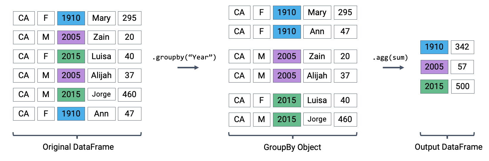
# The code below uses the full babynames dataset, which is why
# some numbers are different relative to the diagram.
babynames[["Year", "Count"]].groupby("Year").agg(sum)
| Count | |
|---|---|
| Year | |
| 1910 | 9163 |
| 1911 | 9983 |
| 1912 | 17946 |
| 1913 | 22094 |
| 1914 | 26926 |
| ... | ... |
| 2018 | 395436 |
| 2019 | 386996 |
| 2020 | 362882 |
| 2021 | 362582 |
| 2022 | 360023 |
113 rows × 1 columns
There are many different aggregation functions we can use, all of which are useful in different applications.
# What is the earliest year in which each name appeared?
babynames.groupby("Name")[["Year"]].agg(min)
| Year | |
|---|---|
| Name | |
| Aadan | 2008 |
| Aadarsh | 2019 |
| Aaden | 2007 |
| Aadhav | 2014 |
| Aadhini | 2022 |
| ... | ... |
| Zymir | 2020 |
| Zyon | 1999 |
| Zyra | 2012 |
| Zyrah | 2011 |
| Zyrus | 2021 |
20437 rows × 1 columns
# What is the largest single-year count of each name?
babynames.groupby("Name")[["Count"]].agg(max)
| Count | |
|---|---|
| Name | |
| Aadan | 7 |
| Aadarsh | 6 |
| Aaden | 158 |
| Aadhav | 8 |
| Aadhini | 6 |
| ... | ... |
| Zymir | 5 |
| Zyon | 17 |
| Zyra | 16 |
| Zyrah | 6 |
| Zyrus | 5 |
20437 rows × 1 columns