Lecture 28 – Data 100, Fall 2023

Data 100, Fall 2023

Acknowledgments Page

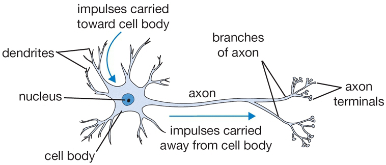
Neurons pass information from one to another using action potentials. They connect with one another at synapses, which are junctions between one neuron's axon and another's dendrite. Information flows from:

1. The dendrites,
2. To the cell body,
3. Through the axons,
4. To a synapse connecting the axon to the dendrite of the next neuron.

An Artificial Neuron is a mathematical function with the following elements:

1. Input
2. Weighted summation of inputs
3. Processing unit of activation function
4. Output

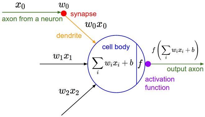
The mathematical equation for an artificial is as follows:

\begin{align} \hat{y} = f(\vec{\mathbf{\theta}} \cdot \vec{\mathbf{x}}) &= f(\sum_{i=0}^d \theta_i x_i) \\ &= f(\theta_0 + \theta_1 x_1 + ... + \theta_dx_d). \end{align}

Assuming that function $f$ is the logistic or sigmoid function, the output of the neuron has a probability value ($0 \leq p \leq 1$). This probability value can then be used for a binary classification task where $p < 0.5$ is an indication of class $0$, and $p \geq 0.5$ assigns data to class 1. Re-writing the equation above with a sigmoid activation function would give us the following:

\begin{align} \hat{y} = σ(\vec{\mathbf{\theta}} \cdot \vec{\mathbf{x}}) &= σ(\sum_{i=0}^d \theta_i x_i) \\ &= σ(\theta_0 + \theta_1 x_1 + ... + \theta_dx_d). \end{align}

The code below contains an implementation of AND, OR, and XOR gates. You will be able to generate data for each of the functions and add the desired noise level to the data. Familiarize yourself with the code and answer the following questions.

What you will do in teams...

1. Observe the decision boundary of the AND function. Is this similar to what we have discussed in the lecture?
2. Identify the parameters for the OR model. What are $w_0$, $w_1$, and $w_2$ values?
3. What is the decision boundary for the XOR gate? How would you describe your observation from the XOR gate?

import tensorflow as tf
from sklearn.model_selection import train_test_split
from tensorflow.keras.utils import to_categorical
from sklearn.linear_model import LogisticRegression
from plotly.subplots import make_subplots
from mlxtend.plotting import plot_decision_regions
from sklearn.metrics import PrecisionRecallDisplay

import numpy as np
import matplotlib.pyplot as plt
import random
import pandas as pd

2023-11-30 22:18:06.995626: I tensorflow/core/platform/cpu_feature_guard.cc:182] This TensorFlow binary is optimized to use available CPU instructions in performance-critical operations.
To enable the following instructions: SSE4.1 SSE4.2 AVX AVX2 FMA, in other operations, rebuild TensorFlow with the appropriate compiler flags.

Datasets for Logical Gates: Loading and Visualization

###### AND OR XOR Data Generator

def Generator(N, Gate= 'OR', noise = 0.05):
  X = []
  y = []
  values = [0, 1]
  for i in range(0, N):
    x1 = random.choice(values)
    x2 = random.choice(values)
    if Gate=='OR': o = x1 | x2
    if Gate=='AND': o = x1 & x2
    if Gate=='XOR': o = x1 != x2
    X.append([x1, x2])
    y.append(o)

  X = np.asarray(X)
  X = X + np.random.normal(0, noise, X.shape)
  y = np.asarray(y, np.int64)
  return X, y

# Creating a dataset with 500 samples and a given noise level
GATE = 'AND' #@param ["OR", "AND", "XOR"]
Noise = 0.05  #@param {type:"slider", min:0, max:1, step:0.05}

# Converting the label to a categorical variable
X, y = Generator(500, GATE, noise = Noise)
y_binary = to_categorical(y)

# Looking into the data and labels
print("**********Data Shape**********")
print("Shape of X:", X.shape)
print("Shape of y:", y.shape)
print("\n")
print("**********Inputs and Labels samples**********")
print("Sample Inputs:", X[0:5, :], sep='\n')
print("Sample Labels:", y_binary[0:5, :], sep='\n')
print("\n")
# Plotting the data
print("**********Plotting the data**********")
df = pd.DataFrame(dict(x1=X[:, 0], x2=X[:, 1], label=y))
colors = {0: 'red', 1: 'blue'}
fig, ax = plt.subplots()
grouped = df.groupby('label')
for key, group in grouped:
  group.plot(ax=ax, kind='scatter', x='x1', y='x2', label=key, color=colors[key])

plt.show()

**********Data Shape**********
Shape of X: (500, 2)
Shape of y: (500,)


**********Inputs and Labels samples**********
Sample Inputs:
[[ 0.97973418  0.066751  ]
 [ 0.03962024  0.93056634]
 [-0.05234573 -0.07189135]
 [-0.05566325  0.96960733]
 [ 0.05949002 -0.00790428]]
Sample Labels:
[[1. 0.]
 [1. 0.]
 [1. 0.]
 [1. 0.]
 [1. 0.]]


**********Plotting the data**********

Training an Artificial Neuron with a Sigmoid Activation and Plotting the Decision Boundary

# Building a step function classifier with threshold = 0
class classifier:
  def predict(self, y):
    return y >= 0

# Function to perform linear regression classification
def perform_logistic_regression(x, y):
    # Splitting the data and label into training and test sets with 80%-20% ratio
    x_train, x_test, y_train, y_test = train_test_split(x, y, test_size=0.2, random_state=140)

    # Training a logistic regression model on the training data
    model = LogisticRegression().fit(x_train, y_train)

    # Checking the accuracy of the model on both training and test data
    print('Training Score: ', model.score(x_train, y_train))
    print('Testing Score: ', model.score(x_test, y_test))

    # Getting the model's parameters and building the weight vector
    weights = np.concatenate([np.expand_dims(model.intercept_, 1), model.coef_], 1)
    print("Weights: ", weights)
    
    plt.figure(figsize=(10,10))
    # Plotting the decision boundary of the model
    plot_decision_regions(x_train, y_train, clf=model, legend=2)
    # Plotting the test data to check the model's performance
    plt.scatter(x_test[:, 0], x_test[:, 1], c=y_test)
    plt.show()

    

    # Displaying precision-recall curve
    display = PrecisionRecallDisplay.from_estimator(
        model, x_test, y_test, name="Logistic Regression"
    )
    _ = display.ax_.set_title("Precision-Recall curve")


perform_logistic_regression(X, y)

Training Score:  1.0
Testing Score:  1.0
Weights:  [[-7.99192798  4.93901091  5.24713597]]

Remember your responses to the following questions:

1. Observe the decision boundary of the AND function. Is this similar to what we have discussed in the lecture?
2. Identify the parameters for the OR model. What are $w_0$, $w_1$, and $w_2$ values?
3. What is the decision boundary for the XOR gate? How would you describe your observation from the XOR gate?