An Overview of Pandas GroupBy
import numpy as np
import pandas as pd
This exercise is inspired by Wes McKinney's Python for Data Analysis
df = pd.read_csv("elections.csv")
df.head()
Grouping a Series by a Series
Let's group the % Series by the Party Series. A call to groupby does that, but what is the object that results?
percent_grouped_by_party = df['%'].groupby(df['Party'])
type(percent_grouped_by_party)
As we see, percent_grouped_by_party is NOT a familiar object like a DataFrame, Series, or Index. Instead, it's a SeriesGroupBy object. A SeriesGroupBy consists of groups, one for each of the distinct values of the Party column. If we ask to see these groups, we'll be able to see which indices in the original DataFrame correspond to each group.
percent_grouped_by_party.groups
The percent_grouped_by_party object is capable of making computations across all these groups. For example, if we call the mean method of the SeriesGroupBy class, we'll get a new Series containing the mean of the "Democratic" Series, the mean of the "Independent" Series, and the mean of the "Republican" Series.
percent_grouped_by_party.mean()
The output of the mean methood is a regular ole pandas Series.
type(percent_grouped_by_party.mean())
SeriesGroupBy objects have many other handy methods, e.g. max and min.
percent_grouped_by_party.max()
percent_grouped_by_party.min()
percent_grouped_by_party.size()
percent_grouped_by_party.first()
We can iterate over a SeriesGroupBy object -- though we're doing this just for educational purposes and you'll probably never actually do this with a real SeriesGroupBy. As we iterate we get pairs of (name, group), where name is a String label for the group, and group is a Series corresponding to the all the values from the given group.
from IPython.display import display  # like print, but for complex objects

for name, group in percent_grouped_by_party:
    print('Name:', name)
    print(type(group))
    display(group)
Grouping a Series by Multiple Series
We can also group a Series by multiple Series. For example, suppose we want to track all combinations of {'Democratic', 'Republican', and 'Independent'} and {'win', 'loss'}.
percent_grouped_by_party_and_result = df['%'].groupby([df['Party'], df['Result']])
percent_grouped_by_party_and_result.groups
Given this groupby object, we can compute the average percentage earned every time each of the parties won and lost the presidential election. We see that at least between 1980 and 2016, the Republicans have typically lost and won their elections by wider margins.
percent_grouped_by_party_and_result.mean()
The careful reader will note that the returned object looks a little funny. It seems to have two indexes! If we check the type of this object, we'll see it's just a regular Series.
type(percent_grouped_by_party_and_result.mean())
However if we request to see the index of this Series, we see that it is a "MultiIndex", which is a special type of index used for data that is indexed in two or more ways.
percent_grouped_by_party_and_result.mean().index
We won't go into MultiIndexes formally today, but be aware that it is possible to index into a Series that has a MultiIndex. The sytnax is about exactly as you'd expect, for example:
percent_grouped_by_party_and_result.mean()["Democratic"]
Grouping a DataFrame by a Series
We can also group an entire dataframe by one or more Series. This results in a DataFrameGroupBy object as the result:
everything_grouped_by_party = df.groupby('Party')
everything_grouped_by_party
As in our previous example, this object contains three group objects, one for each party label.
everything_grouped_by_party.groups
Just as with SeriesGroupBy objects, we can iterate over a DataFrameGroupBy object to understand what is effectively inside.
for n, g in everything_grouped_by_party:
    print('name:', n)
    display(g)
And just like SeriesGroupBy objects, we can apply methods like mean to compute the mean of each group. Since a DataFrameGroupBy is linked to the entire original dataframe (instead of to a single column from the dataframe), we calculate a mean for every numerical column. In this example below, we get the mean vote earned (as before), and the mean year (which isn't a useful quantity).
everything_grouped_by_party.mean()
Where did all the other columns go in the mean above? They are nuisance columns, which get automatically eliminated from an operation where it doesn't make sense (such as a numerical mean).
Grouping a DataFrame by Multiple Series
DataFrames may also be grouped by multiple series at once. For example, we can repeat what we did with a Series above and group the entire DataFrame by Party and Result. After aggregation, we end up with a DataFrame that has a MultiIndex.
everything_grouped_by_party_and_result=df.groupby([df['Party'], df['Result']])
everything_grouped_by_party_and_result.max()
The resulting DataFrame above is pretty strange. We'll observe that Walter Mondale did not run for office in 2016! Make sure you understand why this is happening, as this sort of thing is a common mistake made by people who don't fully understand how pandas works.
Challenge: Try to figure out how to generate a table like the one above, except that each entry should represent all attributes of the candidate who got the maximum vote in that category. For example, the Republican Win category should feature Reagan in 1984 with 58.8% of the vote. The answer is a few cells below this one. There's a hint a few cells down.
Hint: Consider using sort_values and first somehow.
df.sort_values("%", ascending=False).groupby([df['Party'], df['Result']]).first()
The result of an aggregation function applied to a DataFrameGroupBy
Custom Aggregation Functions
As described above, both SeriesGroupBy and DataFrameGroupBy objects have lots of handy methods for computing aggregate values for groups, e.g.
percent_grouped_by_party.min()
everything_grouped_by_party.median()
It turns out that all of these GroupBy methods are just shorthand for a more powerful and universal method of our GroupBy objects called agg. For example, .min() is just shorthand for .agg(min), where min refers to the function min.
percent_grouped_by_party.agg(min)
Naturally, we can define our own custom aggregation functions. For example, the function below returns the first item in a series.
def average_of_first_and_last(series):
    return (series.iloc[0] + series.iloc[-1])/2
We can supply this function as a custom aggregation function for each series. As you can see, nuisance columns are automatically removed.
everything_grouped_by_party.agg(average_of_first_and_last)
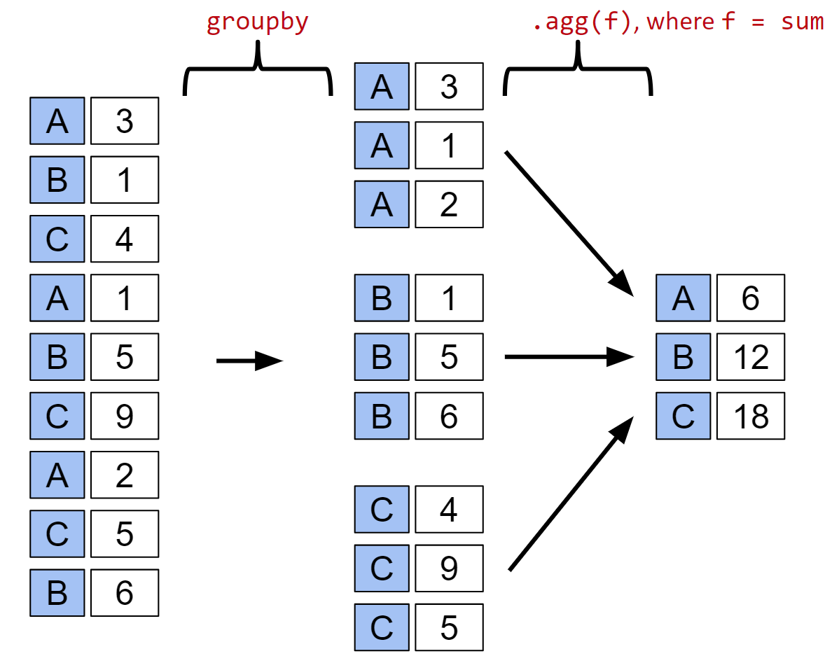
agg is fundamental to our use of GroupBy objects. Indeed, you will rarely call groupby without also calling agg, at least implicitly. We can summarize the grouping process with the following diagram, inspired by a similar diagram created by DS100 instructor Joey Gonzales. Diagram source at this link.

The result of calling groupby then agg on a Series is also a Series, and the result of calling groupby then agg on a DataFrame is also typically a DataFrame, though there are exceptions, e.g. if you use the aggregation function size, you will get back a Series.
def list_of_first_and_last(series):
    return [series.iloc[0], series.iloc[-1]]
everything_grouped_by_party.agg(list_of_first_and_last)
Using Groups to Filter Datasets
everything_grouped_by_party = df.groupby('Party')
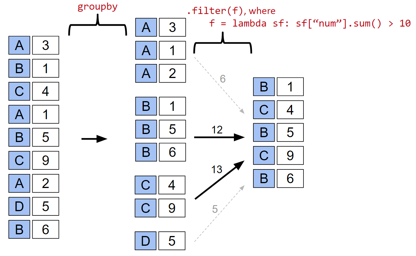
everything_grouped_by_party.filter(lambda subframe: subframe["Year"].max() < 2000)
everything_grouped_by_year = df.groupby('Year')
everything_grouped_by_year.filter(lambda subframe: subframe["%"].sum() < 97)
A visual picture of how filtering works is shown below.

Using isin for filtering
This isn't actually related to groupby at all, but it seemed natural to bring it up here.
Sometimes we want to restrict our attention to only rows where certain values appear. For example, we saw last time how we'd look at only rows that contain "Democratic" candidates.
df[df["Party"] == "Democratic"]
Suppose we wanted to filter such that all Republicans and Democrats appeared. One ugly way to do this would be df[(df["Party"] == "Democratic") | (df["Party"] == "Republican")]. However, a better idea is to use the isin method.
df[(df["Party"] == "Democratic") | (df["Party"] == "Republican")]

df[df["Party"].isin(["Republican", "Democratic"])]
Grouping over a different dimension (bonus topic, less often useful)
Above, we've been grouping data along the rows, using column keys as our selectors. But we can also group along the columns, for example we can group by how many times the letter a appears in the column name.
grouped = df.groupby(lambda x: x.count('a'), axis=1)
for dtype, group in grouped:
    print(dtype)
    display(group)
grouped.max().head(5)
financial_data = pd.read_csv("financial_data.csv", index_col = 0)
financial_data.head(5)
def get_year(datestr):
    return datestr.split('/')[2]
grouped_by_year = financial_data.groupby(get_year, axis=1)
grouped_by_year.mean()
Example from Lecture Figures
For your convenience, we've provided the dataframe from lecture for the groupby examples.
lex = pd.DataFrame({"name": ["A", "B", "C", "A", "B", "C", "A", "D", "B"],
             "num": [3, 1, 4, 1, 5, 9, 2, 5, 6]})
lex.groupby("name").filter(lambda sf: sf["num"].sum() > 10)
Pivot Tables
Recall from before that we were able to group the % Series by the "Party" and "Result" Series, allowing us to understand the average vote earned by each party under each election result.
percent_grouped_by_party_and_result = df['%'].groupby([df['Party'], df['Result']])
percent_grouped_by_party_and_result.mean()
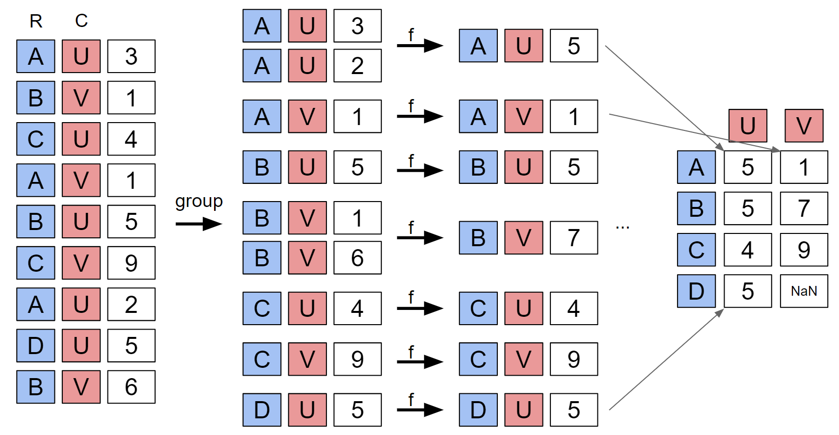
Because we called groupby on a Series, the result of our aggregation operation was also a Series. However, I believe this data is more naturally expressed in a tabular format, with Party as the rows, and Result as the columns. The pivot_table operation is the natural way to achieve this data format.
df_pivot = df.pivot_table(
    index='Party', # the rows (turned into index)
    columns='Result', # the column values
    values='%', # the field(s) to processed in each group
    aggfunc=np.mean, # group operation
)
df_pivot.head()
The basic idea is that you specify a Series to be the index (i.e. rows) and a Series to be the columns. The data in the specified values is then grouped by all possible combinations of values that occur in the index and columns Series. These groups are then aggregated using the aggfunc, and arranged into a table that matches the requested index and columns. The diagram below summarizes how pivot tables are formed. (Diagram inspired by Joey Gonzales). Diagram source at this link.

For more on pivot tables, see this excellent tutorial by Chris Moffitt.
List Arguments to pivot_table (Extra)
The arguments to our pivot_table method can also be lists. A few examples are given below.
If we pivot such that only our columns argument is a list, we end up with columns that are MultiIndexed.
df_pivot = df.pivot_table(
    index='Party', # the rows (turned into index)
    columns=['Result', 'Candidate'], # the column values
    values='%', # the field(s) to processed in each group
    aggfunc=np.mean, # group operation
)
df_pivot.head()
If we pivot such that only our index argument is a list, we end up with rows that are MultiIndexed.
df_pivot = df.pivot_table(
    index=['Party', 'Candidate'], # the rows (turned into index)
    columns='Result',# the column values
    values='%', # the field(s) to processed in each group
    aggfunc=np.mean, # group operation
)
df_pivot
If we pivot such that only our values argument is a list, then we again get a DataFrame with multi-indexed Columns.
df_pivot = df.pivot_table(
    index='Party', # the rows (turned into index)
    columns='Result',# the column values
    values=['%', 'Year'], # the field(s) to processed in each group
    aggfunc=np.mean, # group operation
)
df_pivot
Feel free to experiment with other possibilities!