import numpy as np
import matplotlib.pyplot as plt
import pandas as pd
import seaborn as sns
%matplotlib inline

# ## Plotly plotting support
# import plotly.plotly as py

import plotly.offline as py
py.init_notebook_mode(connected=True)

import plotly.graph_objs as go
import plotly.figure_factory as ff
import cufflinks as cf

cf.set_config_file(offline=False, world_readable=True, theme='ggplot')
Introduction
In this lecture we examine the process of data cleaning and Exploratory Data Analysis (EDA). Often you will acquire or even be given a collection of data in order to conduct some analysis or answer some questions. The first step in using that data is to ensure that it is in the correct form (cleaned) and that you understand its properties and limitations (EDA). Often as you explore data through EDA you will identify additional transformations that may be required before the data is ready for analysis.
In this notebook we obtain crime data from the city of Berkeley's public records. Ultimately, our goal might be to understand policing patterns but before we get there we must first clean and understand the data.
Unboxing the Data
We have downloaded some data from the city of Berkeley's open data repositories and placed them in the data folder. The first step to understanding the data is learning a bit about the files.
How big is the data?
I often like to start my analysis by getting a rough estimate of the size of the data. This will help inform the tools I use and how I view the data. If it is relatively small I might use a text editor or a spreadsheet to look at the data. If it is larger, I might jump to more programmatic exploration or even used distributed computing tools.
The following command lists (l) the files with human (h) readable file sizes:
ls -lh data
In some file systems addition attributes describing the file may be available:
ls -lh@ data
You may also want to try the file command:
!file data/*
This command reveals a bit more about the structure of the data.
All the files are relatively small and we could comfortable examine them in a text editors. (Personally, I like sublime or emacs but others may prefer a different view.).
In listing the files I noticed that the names suggest that they are all text file formats:
- CSV: Comma separated values is a very standard table format.
- JSON: JavaScript Object Notation is a very standard semi-structured file format used to store nested data.
We will dive into the formats in a moment. However because these are text data I might also want to investigate the number of lines which often correspond to records.
Here I am invoking the shell command via the ! operator. The wc command computes the number of lines, words, and characters in each file:
!wc data/*
If we wanted to learn more about the command we could use the man (short for manual) command to read the manual page for wc (word count).
man wc
What is the format?
We already noticed that the files end in csv and json which suggests that these are comma separated values and javascript object notation files. However, we can't always rely on the naming as this is only a convention. Often files will have incorrect extensions or no extension at all.
Let's assume that these are text files (and do not contain binary encoded data). We could then use the head command to look at the first few lines in each file.
!head -n 7 data/Berkeley_PD_-_Calls_for_Service.csv
What are some observations about Berkeley_PD_-_Calls_for_Service.csv?
- It appears to be in comma separated value (CSV) format.
- First line contains the column headings
- There are "quoted" strings in the
Block_Locationcolumn:
these are going to be difficult. What are the implications on our earlier word count"2500 LE CONTE AVE Berkeley, CA (37.876965, -122.260544)"wccalculation?
Examining the rest of the files:
!head -n 5 data/cvdow.csv
The cvdow.csv file is relatively small. We can use the cat command to print out the entire file:
!cat data/cvdow.csv
Seems like a pretty standard well formatted CSV file.
Finally examining the stops.json file:
!head data/stops.json
Observations?
This appears to be a fairly standard JSON file. We notice that the file appears to contain a description of itself in a field called "meta" (which is presumably short for meta-data). We will come back to this meta data in a moment but first let's quickly discuss the JSON file format.
A quick note on JSON
JSON (JavaScript Object Notation) is a common format for exchanging complex structured and semi-structured data.
{
    "field1": "value1",
    "field2": ["list", "of", "values"],
    "myfield3": {"is_recursive": true, "a null value": null}
}
A few key points:
- JSON is a recursive format in that JSON fields can also contain JSON objects
- JSON closely matches Python Dictionaries:
d = {
  "field1": "value1",
  "field2": ["list", "of", "values"],
  "myfield3": {"is_recursive": True, "a null value": None}
}
print(d['myfield3'])
- Very common in web technologies (... JavaScript)
- Many languages have tools for loading and saving JSON objects
Loading the Data
We will now attempt to load the data into python. We will be using the Pandas dataframe library for basic tabular data analysis. Fortunately, the Pandas library has some relatively sophisticated functions for loading data.
cvdow = pd.read_csv("data/cvdow.csv")
cvdow
This dataset is a dictionary which has a clear primary key CVDOW. We will therefore set the index when loading the file.
cvdow = pd.read_csv("data/cvdow.csv").set_index("CVDOW")
cvdow
Looks like a dictionary that defines the meaning of values for a field stored in another table.
Loading the Calls Data
Because the file appears to be a relatively well formatted CSV we will attempt to load it directly and allow the Pandas Library to deduce column headers. (Always check that first row and column look correct after loading.)
calls = pd.read_csv("data/Berkeley_PD_-_Calls_for_Service.csv")
calls.head()
How many records did we get?
len(calls)
Preliminary observations on the data?
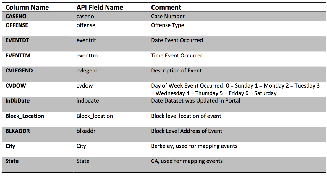
EVENTDT-- Contain the incorrect time stampEVENTTM-- Contains the time in 24 hour format (What timezone?)InDbDate-- Appears to be correctly formatted and appears pretty consistent in time.Block_Location-- Errr, what a mess! newline characters, and Geocoordinates all merged!! Fortunately, this field was "quoted" otherwise we would have had trouble parsing the file. (why?)BLKADDR-- This appears to be the address in Block Location.CityandStateseem redundant given this is supposed to be the city of Berkeley dataset.
calls.drop("Day", axis=1, inplace=True, errors='ignore')
calls['Day'] = calls.join(cvdow, on='CVDOW')['Day']
calls.head()
Checking that City and State are Redundant
We notice that there are city and state columns. Since this is supposed to be data for the city of Berkeley these columns appear to be redundant. Let's quickly compute the number of occurences of unique values for these two columns.
calls.groupby(["City", "State"]).count()
Cleaning Block Location
The block location contains the GPS coordinates and I would like to use these to analyze the location of each request. Let's try to extract the GPS coordinates using regular expressions (we will cover regular expressions in future lectures):
calls_lat_lon = (
    # Remove newlines
    calls['Block_Location'].str.replace("\n", "\t")
    # Extract Lat and Lon using regular expression
    .str.extract(".*\((?P<Lat>\d*\.\d*)\, (?P<Lon>-?\d*.\d*)\)",expand=True)
)
calls_lat_lon.head()
The following block of code joins the extracted Latitude and Longitude fields with the calls data. Notice that we actually drop these fields before joining. This is to enable repeated invocation of this cell even after the join has been completed. (Not necessary but a good habit.)
# Remove Lat and Lon if they already existed before (reproducible)
calls.drop(["Lat", "Lon"], axis=1, inplace=True, errors="ignore")
# Join in the the latitude and longitude data
calls = calls.join(calls_lat_lon)
calls.head()
Python has relatively good support for JSON data since it closely matches the internal python object model.
In the following cell we import the entire JSON datafile into a python dictionary.
import json

with open("data/stops.json", "rb") as f:
    stops_json = json.load(f)
The stops_json variable is now a dictionary encoding the data in the file:
type(stops_json)
We can now examine what keys are in the top level json object
We can list the keys to determine what data is stored in the object.
stops_json.keys()
Observation
The JSON dictionary contains a meta key which likely refers to meta data (data about the data). Meta data often maintained with the data and can be a good source of additional information.
Digging into Meta Data
We can investigate the meta data further by examining the keys associated with the metadata.
stops_json['meta'].keys()
The meta key contains another dictionary called view. This likely refers to meta-data about a particular "view" of some underlying database. We will learn more about views as we study SQL later in the class.
stops_json['meta']['view'].keys()
Notice that this a nested/recursive data structure. As we dig deeper we reveal more and more keys and the corresponding data:
meta
|-> data
    | ... (haven't explored yet)
|-> view
    | -> id
    | -> name
    | -> attribution
    ...
There is a key called description in the view sub dictionary. This likely contains a description of the data:
print(stops_json['meta']['view']['description'])
Columns Meta data
Another potentially useful key in the meta data dictionary is the columns. This returns a list:
type(stops_json['meta']['view']['columns'])
We can brows the list using python:
for c in stops_json['meta']['view']['columns']:
    print(c["name"], "----------->")
    if "description" in c:
        print(c["description"])
    print("======================================\n")
- The above meta data tells us a lot about the columns in the data including both column names and even descriptions. This information will be useful in loading and working with the data.
- JSON makes it easier (than CSV) to create "self-documented data".
- Self documenting data can be helpful since it maintains it's own description and these descriptions are more likely to be updated as data changes.
stops_json['data'][0:2]
Building a Dataframe from JSON
In the following block of code we:
- Translate the JSON records into a dataframe
- Remove columns that have no metadata description. This would be a bad idea in general but here we remove these columns since the above analysis suggests that they are unlikely to contain useful information.
- Examine the top of the table
# Load the data from JSON and assign column titles
stops = pd.DataFrame(
    stops_json['data'],
    columns=[c['name'] for c in stops_json['meta']['view']['columns']])

# Remove columns that are missing descriptions
bad_cols = [c['name'] for c in stops_json['meta']['view']['columns'] if "description" not in c]

# Note we make changes in place
#  This is generally a bad idea but since the stops dataframe is
#  created in the same cell it will be ok.
stops.drop(bad_cols, axis=1, inplace=True)


stops.head()
Preliminary Observations
What do we observe so far?
We observe:
- The
Incident Numberappears to have the year encoded in it. - The
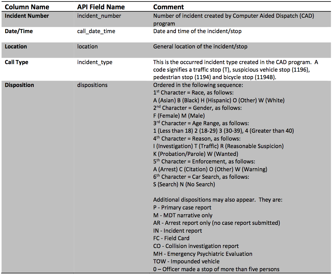
Call Date/TimeField looks to be formatted in YYYY-MM-DDTHH:MM:SS. I am guessing T means "Time". Incident Typehas some weird coding. This is define in the column meta data: This is the occurred incident type created in the CAD program. A code signifies a traffic stop (T), suspicious vehicle stop (1196), pedestrian stop (1194) and bicycle stop (1194B).
EDA
Now that we have loaded our various data files. Let's try to understand a bit more about the data by examining properties of individual fields.
EDA on the Calls Data
calls.head()
Checking that City and State are Redundant
We notice that there are city and state columns. Since this is supposed to be data for the city of Berkeley these columns appear to be redundant. Let's quickly compute the number of occurences of unique values for these two columns.
calls.groupby(["City", "State"]).count()
Are Case Numbers unique?
Case numbers are probably used internally to track individual cases and my reference other data we don't have access to. However, it is possible that multiple calls could be associated with the same case. Let's see if the case numbers are all unique.
print("There are", len(calls['CASENO'].unique()), "unique case numbers.")
print("There are", len(calls), "calls in the table.")
Are case numbers assigned consecutively.
calls['CASENO'].sort_values().reset_index(drop=True).plot()
plt.xlabel("Ordered Location in Data")
plt.ylabel("Case Number")

I like to use interactive plotting tools so I can hover the mouse over the plot and read the values. The cufflinks library adds plotly support to Pandas.
calls['CASENO'].sort_values().reset_index(drop=True).iplot(
    xTitle="Ordered Location in Data",
    yTitle="Case Number",
    layout = dict(yaxis=dict(hoverformat="d")))
Examining the distribution of case numbers shows a similar pattern
calls['CASENO'].iplot(kind="hist",bins=100)
What might we be observing?
One possible explanation is that case numbers were assigned consecutively and then sampled uniformly at different rates for two different periods. We will be able to understand this better by looking at the dates on the cases.
Examining the Date
Given the weird behavior with the case numbers let's dig into the date in which events were recorded. Notice in this data we have several pieces of date/time information (this is not uncommon):
EVENTDT: This contains the date the event took place. While it has time information the time appears to be00:00:00.EVENTTM: This contains the time at which the event took place.InDbDate: This appears to be the date at which the data was entered in the database.
calls.head(3)
When Pandas loads more complex fields like dates it will often load them as strings:
calls["EVENTDT"][0]
We will want to convert these to dates. Pandas has a fairly sophisticated function pd.to_datetime which is capable of guessing reasonable conversions of dates to date objects.
dates = pd.to_datetime(calls["EVENTDT"])
We can verify that the translations worked by looking at a few dates:
pd.DataFrame(dict(transformed=dates, original=calls["EVENTDT"])).head()
We can also extract the time field:
times = pd.to_datetime(calls["EVENTTM"]).dt.time
times.head()
To combine the correct date and correct time field we use the built-in python datetime combine function.
from datetime import datetime
timestamps = pd.to_datetime(pd.concat([dates, times], axis=1).apply(
    lambda r: datetime.combine(r['EVENTDT'], r['EVENTTM']), axis=1))
timestamps.head()
We now updated calls to contain this additional informations:
calls['timestamp'] = timestamps
calls.head()
What time range does the data represent
calls['timestamp'].min()
calls['timestamp'].max()
(
    calls
        .sort_values('timestamp')
        .iplot(
            mode='markers', size=5,
            x='timestamp', y='CASENO',
            xTitle="Ordered Location in Data",
            yTitle="Case Number",
            layout = dict(yaxis=dict(hoverformat="d")))
)
Explanation?
Perhaps there are multiple different record books with different numbering schemes? This might be something worth investigating further.
Are there any other interesting temporal patterns
Do more calls occur on a particular day of the week?
calls['timestamp'].dt.dayofweek.value_counts().iplot(kind='bar', yTitle="Count")
help(pd.Series.dt.dayofweek)
Modified version with dates:
dow = ["Monday", "Tuesday", "Wednesday", "Thursday", "Friday", "Saturday", "Sunday"]

(
    pd.concat([
        pd.Series(dow, name="dow"),
        calls['timestamp'].dt.dayofweek.value_counts()],
        axis=1)
    .set_index("dow")
    .iplot(kind="bar", yTitle="Count")
)
We can check against the day of the week field we added:
(
    calls['Day'].value_counts()[dow]
    .iplot(kind="bar", yTitle="Count")
)
How about temporal patterns within a day?
ts = calls['timestamp']
minute_of_day = ts.dt.hour * 60 + ts.dt.minute
hour_of_day = minute_of_day / 60.

calls['minute_of_day'] = minute_of_day
calls['hour_of_day'] = hour_of_day
py.iplot(ff.create_distplot([hour_of_day],group_labels=["Hour"],bin_size=1))
Observations?
In the above plot we see the standard pattern of limited activity early in the morning around here 6:00AM.
Smoothing Parameters
In the above plot we see a smoothed curve approximating the histogram. This is an example of a kernel density estimator (KDE). The KDE, like the histogram, has a parameter that determines it's smoothness. Many packages (Plotly and Seaborn) use a boostrap like procedure to choose the best value.
To understand how this parameter works we will use seaborn which let's you also set the parameter manually.
sns.distplot(hour_of_day, kde_kws=dict(bw=.1), rug=False)

Notice in the above plot that the interpolation tries to follow the histogram to closely.
Stratified Analysis
To better understand the time of day a report occurs we could stratify the analysis by the day of the week. To do this we will use box plots.
## Using Pandas built in box plot
# calls['hour_of_day'] = minute_in_day
# calls.boxplot('hour_of_day', by='Day')
groups = calls.groupby("CVDOW")
py.iplot([go.Box(y=df["hour_of_day"], name=str(cvdow.loc[i][0])) for (i, df) in groups])
Observations?
There are no very clear patterns here. It is possible Fridays might have crimes shifted slightly more to the evening. In general the time a crime is reported seems fairly consistent throughout the week.
# fig = ff.create_violin(calls, data_header='hour_of_day', group_header='Day')
# py.iplot(fig, filename='Multiple Violins')
calls.head()
The Offense Field
The Offense field appears to contain the specific crime being reported. As nominal data we might want to see a summary constructed by computing counts of each offense type:
calls['OFFENSE'].value_counts().iplot(kind="bar")
Observations?
Car burglary and misdemeanor theft seem to be the most common crimes with many other types of crimes occurring rarely.
CVLEGEND
The CVLEGEND filed provides the broad category of crime and is a good mechanism to group potentially similar crimes.
calls['CVLEGEND'].value_counts().iplot(kind="bar")
Notice that when we group by the crime time we see that larceny becomes the dominant category. Larceny is essentially stealing -- taking someone else stuff without force.
Stratified Analysis of Time of Day by CVLEGEND
View the crime time periods broken down by crime type:
boxes = [(len(df), go.Box(y=df["hour_of_day"], name=i)) for (i, df) in calls.groupby("CVLEGEND")]
py.iplot([r[1] for r in sorted(boxes, key=lambda x:x[0], reverse=True)])
Examining Location information
Let's examine the geographic data (latitude and longitude). Recall that we had some missing values. Let's look at the behavior of these missing values according to crime type.
missing_lat_lon = calls[calls[['Lat', 'Lon']].isnull().any(axis=1)]
missing_lat_lon['CVLEGEND'].value_counts().iplot(kind="bar")
Observations?
There is a clear bias towards drug violations that is not present in the original data. Therefore we should be careful when dropping missing values!
We might further normalize the analysis by the frequency to find which type of crime has the highest proportion of missing values.
(
    missing_lat_lon['CVLEGEND'].value_counts() / calls['CVLEGEND'].value_counts()
).sort_values(ascending=False).iplot(kind="bar")
Day of Year and Missing Values:
We might also want to examine the time of day in which latitude and longitude are missing:
ts = calls['timestamp']

py.iplot(ff.create_distplot([calls['timestamp'].dt.dayofyear,
                             missing_lat_lon['timestamp'].dt.dayofyear],
                            group_labels=["all data", "missing lat-lon"],bin_size=2))
Observations?
Pretty similar
!pip install --upgrade folium
import folium
print(folium.__version__, "should be at least 0.3.0")
import folium
import folium.plugins # The Folium Javascript Map Library

SF_COORDINATES = (37.87, -122.28)
sf_map = folium.Map(location=SF_COORDINATES, zoom_start=13)
locs = calls[['Lat', 'Lon']].astype('float').dropna().as_matrix()
heatmap = folium.plugins.HeatMap(locs.tolist(), radius = 10)
sf_map.add_child(heatmap)
cluster = folium.plugins.MarkerCluster()
for _, r in calls[['Lat', 'Lon', 'CVLEGEND']].dropna().sample(1000).iterrows():
    cluster.add_child(
        folium.Marker([float(r["Lat"]), float(r["Lon"])], popup=r['CVLEGEND']))

sf_map = folium.Map(location=SF_COORDINATES, zoom_start=13)
sf_map.add_child(cluster)
sf_map