🗳️ Lecture 9 – Data 100, Spring 2025

Data 100, Spring 2025

Acknowledgments Page

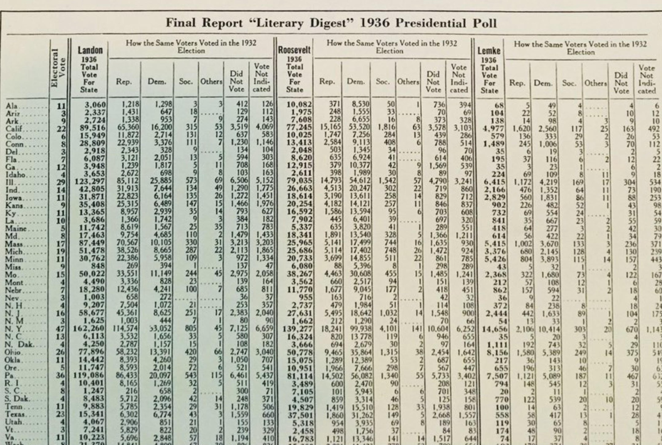
The picture above shows the poll results printed in Literary Digest in 1936. You might think about how tedious it would be to tabulate 2.4 million responses and organize the results in this table by hand. We will use this data later in the demo.

import matplotlib.pyplot as plt
import numpy as np
import pandas as pd
import seaborn as sns
import zipfile

sns.set_theme(style='darkgrid', font_scale = 1.5,
              rc={'figure.figsize':(7,5)})

🇺🇸 1936 Presidential Election Results

Let's start with the real election results from the 1936 election.

• Each row of votes represents a single voter.
• voted_dem is 0/1 variable indicating whether the voter voted for Franklin D. Roosevelt, who was the Democratic candidate in 1936. If 0, the voter voted for Alf Landon, the Republican candidate.

Votes for other parties are excluded from this dataset.

# The large CSV containing all the votes is compressed to reduce storage size.
# This code unzips the file and reads the CSV into a pandas DataFrame.
# No need to be familiar with the unzipping code for Data 100!
with zipfile.ZipFile("1936_votes.zip", 'r') as z:
    with z.open("1936_votes.csv") as csv_file:
        votes = pd.read_csv(csv_file)

votes.head()

	voted_dem
0	1
1	1
2	0
3	1
4	1

How many votes were cast for either Roosevelt or Landon in 1936?

len(votes)

44430549

What fraction of voters voted for Roosevelt, the Democratic candidate?

votes['voted_dem'].sum() / len(votes)

0.6245897614274358

But wait, don't the slides say that Roosevelt won 61% of the vote?

Yes! But, he won 61% of all votes. If we filter to just the voters who voted for Roosevelt or Landon, Roosevelt won 62.5% of votes.

Useful tip: The mean of a 0/1 column is the same as the proportion of values that are 1.

votes['voted_dem'].mean()

0.6245897614274358

Of the 44,430,549 voters who voted for either Roosevelt or Landon, 62.5% voted for Roosevelt.

🎩 Simple Random Sample (SRS)

Note: An SRS is sometimes called a "names in a hat" sample, since it's a lot like putting each observation on a slip of paper, putting all the slips in a big hat, and then randomly drawing slips one at a time.

If we were to take a simple random sample of just 1,000 voters and calculate the proportion who planned to vote for Roosevelt, how close would we be to 62.5%?

votes['voted_dem'].sample(1000).mean()

0.649

Note that the cell above is a little slow, since we're sampling from a DataFrame with almost 45 million rows.

We can speed up the sampling using NumPy:

# Construct a random number generator object.
# No need to be familiar with using NumPy this way in Data 100!
rng = np.random.default_rng()

n_votes = len(votes)

# Generate 1000 random integers from 0 to (number of votes - 1)
idx = rng.integers(low=0, high=n_votes-1, size=1000)

votes['voted_dem'].iloc[idx].mean()

0.618

Both of the estimates above are pretty close to 62.5%! They are much closer than the estimate from the Literary Digest poll, which predicted that 43% of votes would go to Roosevelt.

This is no fluke! If we repeat this over and over, we tend to hover around 62.5%.

for _ in range(10):
  idx = rng.integers(low=0, high=n_votes-1, size=1000)
  print(votes['voted_dem'].iloc[idx].mean())

0.62
0.642
0.648
0.634
0.625
0.617
0.631
0.641
0.616
0.641

Let's randomly generate 10,000 estimates:

nrep = 10000   # number of simulations
n = 1000       # size of our sample
results = []   # list to store the sampling results

for i in range(0, nrep):
    idx = rng.integers(low=0, high=n_votes, size=1000)
    results.append(votes['voted_dem'].iloc[idx].mean())

# First 10 simulated sample proportions
results[:10]

[0.625, 0.631, 0.613, 0.642, 0.628, 0.626, 0.622, 0.641, 0.613, 0.637]

Plotting our estimates with KDE:

plt.figure(figsize=(12, 3))
p = sns.histplot(x=results, kde=True, bins=10)

# Make x-axis centered at 0.625 with 0.01 intervals
p.set_xticks(np.arange(0.625 - 5 * 0.01, 0.625 + 5 * 0.01, 0.01));

We get an approximate normal distribution centered around 62.5%, with most of the mass of the distribution (say, 95% of the mass) within about 3 percentage points (0.03) on each side.

As it turns out, with a sample size of 1000, our estimate of the proportion of voters supporting Roosevelt has a margin of error of about 3 percentage points (3pp) at a 95% confidence level (CL), so long as we take a simple random sample (SRS) of actual voters.

• Note: You tend to see 3pp and 95% CL quite a lot in political polling!

We'll learn what these values mean and how to calculate them when we (re)learn the Central Limit Theorem later in the semester.

Instructor Note: Return to slides!

⏪ Revisiting the 1936 Literary Digest Poll

The poll DataFrame contains a summary of the 1936 Literary Digest Poll, along with polling results and actual election results from 1932 and 1936.

• Each row of poll represents a U.S. state.
• state: name of the U.S. state.
• electoral_votes: # electoral votes allocated to the given state.
• actual_dem_1936: # votes for Roosevelt (the Democratic candidate) in 1936.
• actual_rep_1936: # votes for Landon (the Republican candidate) in 1936.
• ld_dem_1936: # Literary Digest respondents who planned to vote for Roosevelt in 1936.
• ld_rep_1936: # Literary Digest respondents who plannted to vote for Landon in 1936.

Literary Digest also had a 1932 poll! We will use this data for post-stratification:

• actual_dem_1932: # votes for the Democratic candidate in 1932.
• actual_rep_1932: # votes for the Republican candidate in 1932.
• ld_dem_1932: # of 1936 Literary Digest respondents who voted for the Democratic candidate in 1932.
• ld_rep_1932: # of 1936 Literary Digest respondents who voted for Republican candidate in 1932.

Note: Votes from parties other than Democratic and Republican are excluded from this dataset.

poll = pd.read_csv('literary-digest-summary-data.csv')
poll.head()

	state	electoral_votes	actual_dem_1936	actual_rep_1936	ld_rep_1936	ld_dem_1936	actual_dem_1932	actual_rep_1932	ld_dem_1932	ld_rep_1932
0	Alabama	11	238196	35358	3060	10082	207910	34675	9828	1589
1	Arizona	3	86722	33433	2337	1975	79264	36104	2202	1679
2	Arkansas	9	146765	32049	2724	7608	189602	28467	7608	1566
3	California	22	1766836	836431	89516	77245	1324157	847902	69720	80525
4	Colorado	6	295021	181267	15949	10025	250877	189617	9970	13619

As a sanity check, let's make sure we have the same number of votes as the first dataset (44,430,549):

poll['actual_dem_1936'].sum() + poll['actual_rep_1936'].sum()

44430549

Let's also check that we get the reported Literary Digest prediction of 43% for Roosevelt.

• Remember, Roosevelt received 62.5% of the actual vote.

poll['ld_dem_1936'].sum() / (poll['ld_dem_1936'].sum() + poll['ld_rep_1936'].sum())

0.4289439704056572

🥞 Post-stratification with Literary Digest responses from 1932 and 1936

Using post-stratification, let's see if we can improve the Literary Digest poll result using the same information available to Literary Digest in 1936.

• In other words, without using data from the future!

Recall the steps of post-stratification:

1. Divide the sample and population into cells defined by chosen characteristics.
2. Calculate the overall response in each sample cell.
3. Aggregate over sample cells, reweighting by the size of the corresponding population cell.

Sample: Responses to the Literary Digest poll from 1932, among 1936 poll respondents

Population: The actual election outcomes in 1932

Cells: Every combination of state and political party

Wait, aren't we interested in the 1936 Literary Digest poll?

• Yes! But, we can use responses from the older 1932 poll and 1932 election results to get our sample cell weights, and then use these weights to turn the 1936 poll results into a prediction of the 1936 election results.

• Note that this approach assumes that over- and under-representation of voters among the poll respondents in state and party is the same in 1932 and 1936!

Let's start with step 1. We divide our population and sample into cells defined by each combination of state and choice of party in 1932:

• Cell 1: Alabama + Republican in 1932
• Cell 2: Alabama + Democratic in 1932
• Cell 3: Arizona + Republican in 1932
• Cell 4: Arizona + Democratic in 1932
• ...

Note: Alaska and Hawaii were not U.S. states until after 1936.

The population cells are already in polls: actual_dem_1932 and actual_rep_1932 provide the actual vote counts for each party and state in 1932.

The sample cells are also in polls: ld_dem_1932 and ld_rep_1932 provide the number of responses to the 1932 Literary Digest poll, among 1936 poll respondents, for each party.

Let's make the big assumption that respondents in ld_dem_1932 are representative of all voters in actual_dem_1932 for each state, and the same for ld_rep_1932 and actual_rep_1932.

• In other words, we claim that response rates and outreach for Democrats and Republicans from each state in 1932 can differ, but ultimately poll respondents from a particular party+state combination are representative of actual voters for each party+state combination.

• Then, we can calculate the reweighting factor, or how over- or under-represented poll respondents are relative to actual voters.

• All we need to do is divide the actual vote counts by the corresponding number of respondents, for each combination of party and state.

poll['dem_reweight_factor'] = poll['actual_dem_1932'] / poll['ld_dem_1932']
poll['rep_reweight_factor'] = poll['actual_rep_1932'] / poll['ld_rep_1932']
poll.tail()

	state	electoral_votes	actual_dem_1936	actual_rep_1936	ld_rep_1936	ld_dem_1936	actual_dem_1932	actual_rep_1932	ld_dem_1932	ld_rep_1932	dem_reweight_factor	rep_reweight_factor
43	Virginia	11	234980	98336	10223	16783	203979	89637	16194	6817	12.595961	13.149039
44	Washington	8	459579	206892	21370	15300	353260	208645	16223	17122	21.775257	12.185784
45	West Virginia	8	502582	325358	13660	10235	405124	330731	10818	11338	37.449066	29.170136
46	Wisconsin	12	802984	380828	33796	20781	707410	347741	24073	25731	29.386034	13.514477
47	Wyoming	3	62624	38739	2526	1533	54370	39583	1654	2072	32.871826	19.103764

Note that dem_reweight_factor is about 36 for Arizona.

• In other words, there were 36 times as many Democratic voters in Arizona than Democratic poll respondents.

Similarly, rep_reweight_factor is about 21.5 for Arizona.

• So, Democratic voters are underrepresented in the 1932 Literary Digest poll responses, relative to Republican voters.

• Based on the Republican bias in the Literary Digest sample discussed in lecture (i.e., wealthier folks with phones, cars, and magazines), this is expected!

Next, we apply these same weights to inflate the 1936 poll results into vote predictions.

• Again, note that this approach assumes over- and under-representation patterns are the same in the 1932 and 1936 polls!

poll['pred_dem_1936'] = round(poll['ld_dem_1936'] * poll['dem_reweight_factor'])
poll['pred_rep_1936'] = round(poll['ld_rep_1936'] * poll['rep_reweight_factor'])
poll.head()

	state	electoral_votes	actual_dem_1936	actual_rep_1936	ld_rep_1936	ld_dem_1936	actual_dem_1932	actual_rep_1932	ld_dem_1932	ld_rep_1932	dem_reweight_factor	rep_reweight_factor	pred_dem_1936	pred_rep_1936
0	Alabama	11	238196	35358	3060	10082	207910	34675	9828	1589	21.154864	21.821901	213283.0	66775.0
1	Arizona	3	86722	33433	2337	1975	79264	36104	2202	1679	35.996367	21.503276	71093.0	50253.0
2	Arkansas	9	146765	32049	2724	7608	189602	28467	7608	1566	24.921399	18.178161	189602.0	49517.0
3	California	22	1766836	836431	89516	77245	1324157	847902	69720	80525	18.992499	10.529674	1467076.0	942574.0
4	Colorado	6	295021	181267	15949	10025	250877	189617	9970	13619	25.163190	13.922975	252261.0	222058.0

Finally, let's calculate the proportion of predicted votes that are allocated to Roosevelt in 1936.

• Remember that Roosevelt received 62.5% of the actual vote in 1936.

poll['pred_dem_1936'].sum() / (poll['pred_dem_1936'].sum() + poll['pred_rep_1936'].sum())

0.5422251022375592

54% is a majority! Using post-stratification, we have shifted the Literary Digest prediction of a Roosevelt loss with 43% of the vote to a (correct) Roosevelt win with 54%.

• There is no cheating here; we used the same data available to Literary Digest in 1936.

• Note that post-stratification is not perfect. We are still off by almost 10 percentage points. But, we've moved in the right direction.

🎁 Bonus: Follow Up Improvements

As a follow-up exercise, we can compare the predicted 1936 vote totals to the actual 1932 vote totals.

• Then, we could apply a correction factor to change the predicted number of 1936 votes to be in line with the total number of votes in 1932.

• This exercise assumes that the total number of votes cast in 1932 would be the same in 1936, but the poll response rates and outreach might change between 1932 and 1936.

poll['pred_total_1936'] = poll['pred_dem_1936'] + poll['pred_rep_1936']
poll['actual_total_1932'] = poll['actual_dem_1932'] + poll['actual_rep_1932']
poll['correction_factor'] = poll['actual_total_1932'] / poll['pred_total_1936']
poll.head()

	state	electoral_votes	actual_dem_1936	actual_rep_1936	ld_rep_1936	ld_dem_1936	actual_dem_1932	actual_rep_1932	ld_dem_1932	ld_rep_1932	dem_reweight_factor	rep_reweight_factor	pred_dem_1936	pred_rep_1936	pred_total_1936	actual_total_1932	correction_factor
0	Alabama	11	238196	35358	3060	10082	207910	34675	9828	1589	21.154864	21.821901	213283.0	66775.0	280058.0	242585	0.866196
1	Arizona	3	86722	33433	2337	1975	79264	36104	2202	1679	35.996367	21.503276	71093.0	50253.0	121346.0	115368	0.950736
2	Arkansas	9	146765	32049	2724	7608	189602	28467	7608	1566	24.921399	18.178161	189602.0	49517.0	239119.0	218069	0.911969
3	California	22	1766836	836431	89516	77245	1324157	847902	69720	80525	18.992499	10.529674	1467076.0	942574.0	2409650.0	2172059	0.901400
4	Colorado	6	295021	181267	15949	10025	250877	189617	9970	13619	25.163190	13.922975	252261.0	222058.0	474319.0	440494	0.928687

poll['pred_dem_1936_corrected'] = poll['pred_dem_1936'] * poll['correction_factor']
poll['pred_rep_1936_corrected'] = poll['pred_rep_1936'] * poll['correction_factor']

poll['pred_dem_1936_corrected'].sum() / (poll['pred_dem_1936_corrected'].sum() + poll['pred_rep_1936_corrected'].sum())

0.5419440974611633

Looks like a pretty similar prediction for Roosevelt of 54%.

As it turns out, it looks like our original (i.e., uncorrected) predictions had a vote total closer to the true 1936 vote total:

print('Actual 1936 vote total:')
print(poll['actual_dem_1936'].sum() + poll['actual_rep_1936'].sum())

print('Predicted 1936 vote total, uncorrected:')
print(poll['pred_dem_1936'].sum() + poll['pred_rep_1936'].sum())

print('Predicted 1936 vote total, corrected:')
print(poll['pred_dem_1936_corrected'].sum() + poll['pred_rep_1936_corrected'].sum())

Actual 1936 vote total:
44430549
Predicted 1936 vote total, uncorrected:
42058418.0
Predicted 1936 vote total, corrected:
38582531.0

Furthermore, we can check whether post-stratification would have led to a predicted win for Roosevelt in the electoral college, which is what actually determines the election outcome.

• To do this, we allocate all of the electoral votes in each state to the candidate with the most predicted votes in that state, and then sum up the total number of electoral votes allocated to each candidate across states.

poll['dem_wins'] = poll['pred_dem_1936'] > poll['pred_rep_1936']

print('Total predicted Roosevelt electoral votes:')
print(( poll['dem_wins'] * poll['electoral_votes'] ).sum())

print('Total predicted Landon electoral votes:')
print(( (1-poll['dem_wins']) * poll['electoral_votes'] ).sum())

Total predicted Roosevelt electoral votes:
380
Total predicted Landon electoral votes:
151

We (correctly) predict a Roosevelt landslide in the electoral college!

• But, note that the actual electoral college landslide was much bigger: 523 to 8

• This is the largest electoral college landslide since 1820 (as of 2025).