Feature Engineering
In this notebook we will explore a key part of data science, feature engineering: the process of transforming the representation of model inputs to enable better model approximation. Feature engineering enables you to:
- encode non-numeric features to be used as inputs to common numeric models
- capture domain knowledge (e.g., the perceived loudness or sound is the log of the intensity)
- transform complex relationships into simple linear relationships
Overview of Notation for Feature Engineering
The Following video provides an overview of the notation for feature engineering:
from IPython.display import YouTubeVideo
YouTubeVideo("ET44iB169no")
Mapping from Domain to Range
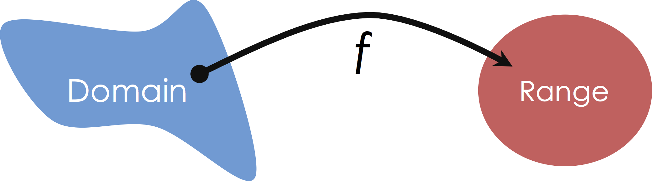
In the past few lectures we have been exploring various models for regression. These are models from some domain to a continuous quantity.
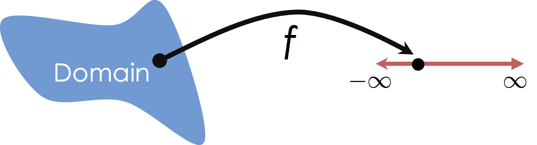
So far we have been interested in modeling relationships from some numerical domain to a continuous quantitative range:
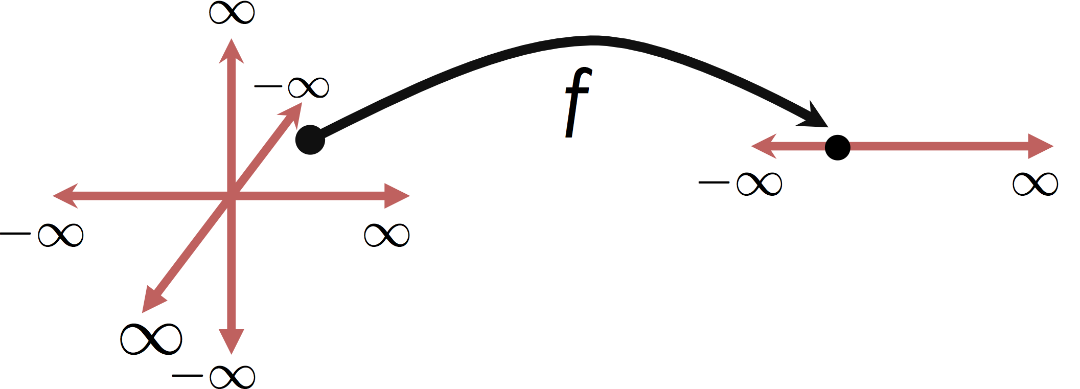
In this class we will focus on Multiple Regression in which we consider mappings from potentially high-dimensional input spaces onto the real line (i.e., $y \in \mathbb{R}$):
It is worth noting that this is distinct from Multivariate Regression in which we are predicting multiple (confusing?) response values (e.g., $y \in \mathbb{R}^q$).
Standard Imports
As usual, we will import a standard set of functions
import numpy as np
import pandas as pd
import plotly.offline as py
import plotly.express as px
import plotly.graph_objects as go
import plotly.figure_factory as ff
import cufflinks as cf
cf.set_config_file(offline=True, sharing=False, theme='ggplot');
from sklearn.linear_model import LinearRegression
Basic Feature Engineering
The following video walks through some of the basic steps in feature engineering as well as the next section of this notebook.
from IPython.display import YouTubeVideo
YouTubeVideo("moL6aeW94Ps")
What does it mean to be a linear model
Linear models are linear combinations of features. These models are therefore linear in the parameters but not necessarily the underlying data. We can encode non-linearity in our data through the use of feature functions:
$$ f_\theta\left( x \right) = \phi(x)^T \theta = \sum_{j=0}^{p} \phi(x)_j \theta_j $$where $\phi$ is an arbitrary function from $x\in \mathbb{R}^d$ to $\phi(x) \in \mathbb{R}^{p+1}$. Notationally, we might right these as a collection of separate feature $\phi_j$ feature functions from $x\in \mathbb{R}^d$ to $\phi_j(x) \in \mathbb{R}$:
$$ \phi(x) = \left[\phi_0(x), \phi_1(x), \ldots, \phi_p(x) \right] $$We often refer to these $\phi_j$ as feature functions and their design plays a critical role in both how we capture prior knowledge and our ability to fit complicated data.
Modeling Non-linear relationships
To demonstrate the power of feature engineering let's return to our earlier synthetic dataset.
synth_data = pd.read_csv("data/synth_data.csv.zip")
synth_data.head()
This dataset is simple enough that we can easily visualize it.
fig = go.Figure()
data_scatter = go.Scatter3d(x=synth_data["X1"], y=synth_data["X2"], z=synth_data["Y"],
                            mode="markers",
                            marker=dict(size=2))
fig.add_trace(data_scatter)
fig.update_layout(margin=dict(l=0, r=0, t=0, b=0),
                  height=600)
fig
Questions:
Is the relationship between $y$ and $x_1$ and $x_2$ linear?
Answer
While the data appear to live on a two dimensional plane there does appear to be some more complex non-linear structure to the data.Previously we fit a linear model to the data using SKlearn
model = LinearRegression()
model.fit(synth_data[["X1", "X2"]], synth_data[["Y"]])
Visualizing the model we obtained:
def plot_plane(f, X, grid_points = 30):
    u = np.linspace(X[:,0].min(),X[:,0].max(), grid_points)
    v = np.linspace(X[:,1].min(),X[:,1].max(), grid_points)
    xu, xv = np.meshgrid(u,v)
    X = np.vstack((xu.flatten(),xv.flatten())).transpose()
    z = f(X)
    return go.Surface(x=xu, y=xv, z=z.reshape(xu.shape),opacity=0.8)
fig = go.Figure()
fig.add_trace(data_scatter)
fig.add_trace(plot_plane(model.predict, synth_data[["X1", "X2"]].to_numpy(), grid_points=5))
fig.update_layout(margin=dict(l=0, r=0, t=0, b=0),
                  height=600)
This wasn't a bad fit but there is definitely more structure.
Designing a Better Feature Function
Examining the above data we see that there is some periodic structure. Let's define a feature function that might try to capture this periodic structure. In the following will add a few different sine functions at different frequences and offsets. Note that for this to remain a linear model, I cannot make the frequence or phase of the sine function a model parameter. Recall in previous lectures we actually made the frequency and phase a parameter of the model and then we were required to used gradient descent to compute the loss minimizing parameter values.
def phi_periodic(X):
    return np.hstack([
        X,
        np.sin(X),
        np.sin(10*X),
        np.sin(20*X),
        np.sin(X + 1),
        np.sin(10*X + 1),
        np.sin(20*X + 1)
    ])
Creating the original $\mathbb{X}$ and $\mathbb{Y}$ matrices
X = synth_data[["X1", "X2"]].to_numpy()
Y = synth_data[["Y"]].to_numpy()
Constructing the $\Phi$ matrix
Phi = phi_periodic(X)
Phi.shape
Fitting the linear model to the transformed features:
model_phi = LinearRegression()
model_phi.fit(Phi, Y)
def predict_phi(X):
    return model_phi.predict(phi_periodic(X))
fig = go.Figure()
fig.add_trace(data_scatter)
fig.add_trace(plot_plane(predict_phi, X, grid_points=100))
fig.update_layout(margin=dict(l=0, r=0, t=0, b=0),
                  height=600)
Examining the model parameters:
model_phi.intercept_ # theta_0
model_phi.coef_ # theta_1 to theta_14
Feature Engineering
The following video gives an overview of standard feature engineering practices.
YouTubeVideo("y6mxtlWYo54")
Feature Functions for Categorical or Text Data
Suppose we are given the following table:
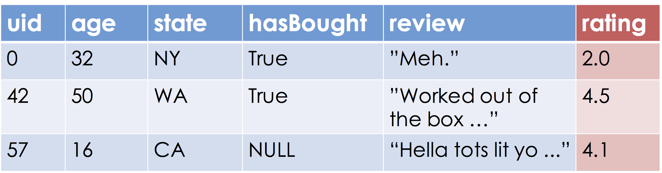
Our goal is to learn a function that approximates the relationship between the blue and red columns. Let's assume the range, "Ratings", are the real numbers (this may be a problem if ratings are between [0, 5] but more on that later).
What is the domain of this function?
The schema of the relational model provides one possible answer:
RatingsData(uid INTEGER, age FLOAT,
            state VARCHAR, hasBought BOOLEAN,
            review VARCHAR, rating FLOAT)
Which would suggest that the domain is then:
integers, real numbers, strings, booleans, and more strings.
Unfortunately, the techniques we have discussed so far and most of the techniques in machine learning and statistics operate on real-valued vector inputs $x \in \mathbb{R}^d$ (or for the statisticians $x \in \mathbb{R}^p$).
Goal:
Moreover, many of these techniques, especially the linear models we have been studying, assume the inputs are qauntitative variables in which the relative magnitude of the feature encode information about the response variable.
In the following we define several basic transformations to encode features as real numbers.
Basic Feature Engineering: Get $\mathbb{R}$
Our first step as feature engineers is to translate our data into a form that encodes each feature as a continuous variable.
The Uninformative Feature: uid
The uid was likely used to join the user information (e.g., age, and state) with some Reviews table. The uid presents several questions:
- What is the meaning of the
uidnumber? - Does the magnitude of the
uidreveal information about the rating?
There are several answers:
Although numbers, identifiers are typically categorical (like strings) and as a consequence the magnitude has little meaning. In these settings we would either drop or one-hot encode the
uid. We will return to feature dropping and one-hot-encoding in a moment.There are scenarios where the magnitude of the numerical
uidvalue contains important information. When user ids are created in consecutive order, larger user ids would imply more recent users. In these cases we might to interpret theuidfeature as a real number and keep it in our model.
Dropping Features
While uncommon there are certain scenarios where manually dropping features might be helpful:
when the features does not to contain information associated with the prediction task. Dropping uninformative features can help to address over-fitting, an issue we will discuss in great detail soon.
when the feature is not available at prediction time. For example, the feature might contain information collected after the user entered a rating. This is a common scenario in time-series analysis.
However, in the absence of substantial domain knowledge, we would prefer to use algorithmic techniques to help eliminate features. We will discuss this in more detail when we return to regularization.
The Continuous age Feature
The age feature encodes the users age. This is already a continuous real number so no additional feature transformations are required. However, as we will soon see, we may introduce additional related features (e.g., indicators for various age groups or non-linear transformations).
The Categorical state Feature
The state feature is a string encoding the category (one of the 50 states). How do we meaningfully encode such a feature as one or more real-numbers?
We could enumerate the states in alphabetical order AL=0, AK=2, ... WY=49. This is a form of dictionary encoding which maps each category to an integer. However, this would likely be a poor feature encoding since the magnitude provides little information about the rating.
Alternatively, we might enumerate the states based on their geographic region (e.g., lower numbers for coastal states.). While this alternative dictionary encoding may provide information there is better way to encode categorical features for machine learning algorithms.
One-Hot Encoding
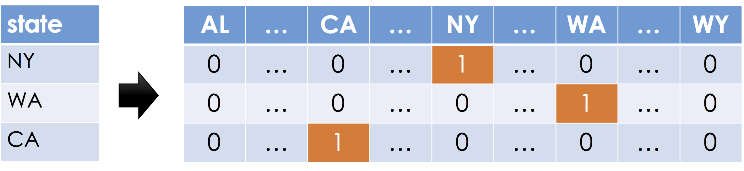
One-Hot encoding, sometimes also called dummy encoding is a simple mechanism to encode categorical data as real numbers such that the magnitude of each dimension is meaningful. Suppose a feature can take on $k$ distinct values (e.g., $k=50$ for 50 states in the United Stated). For each distinct possible value a new feature (dimension) is created. For each record, all the new features are set to zero except the one corresponding to the value in the original feature.
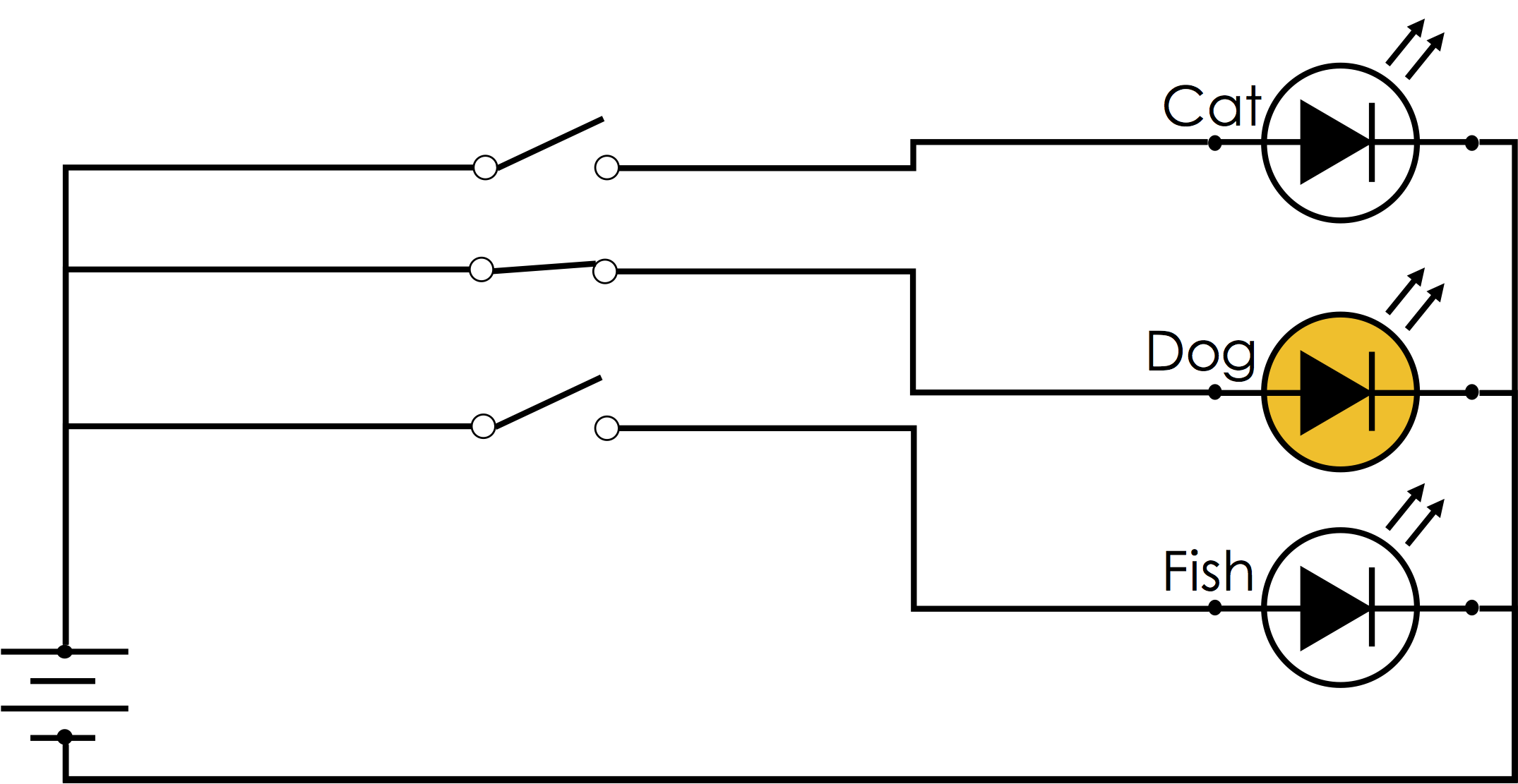
The term one-hot encoding comes from a digital circuit encoding of a categorical state as particular "hot" wire:
One-Hot Encoding in Pandas
Here we create a toy DataFrame of pets including their name and kind:
df = pd.DataFrame({
    "name": ["Goldy", "Scooby", "Brian", "Francine", "Goldy"],
    "kind": ["Fish", "Dog", "Dog", "Cat", "Dog"],
    "age": [0.5, 7., 3., 10., 1.]
}, columns = ["name", "kind", "age"])
df
Pandas has a built in function to construct one-hot encodings called get_dummies
pd.get_dummies(df['kind'])
pd.get_dummies(df)
A serious issue with using Pandas to construct a one-hot-encoding is that if we get new dat in a different DataFrame we may get a different encoding. Scikit-learn provides more flexible routines to construct features.
One-Hot Encoding in Scikit-Learn
Scikit-Learn also has several library for constructing one-hot-encodings. The most basic way to construct a one-hot-encoding is using the scikit-learn OneHotEncoder.
from sklearn.preprocessing import OneHotEncoder

oh_enc = OneHotEncoder()
To "learn" the categories we fit the OneHotEncoder to the data:
oh_enc.fit(df[['name', 'kind']])
We can get the "names" of the new one-hot-encoding columns which reveal both the source columns and the categories within each column:
oh_enc.get_feature_names()
We can also construct the OneHotEncoding of the data:
oh_enc.transform(df[['name', 'kind']])
Notice that the One-Hot-Encoding produces a sparse output matrix. This is because most the entries are 0. If we wanted to see the matrix we could do one of the following:
oh_enc.transform(df[['name', 'kind']]).todense()
import matplotlib.pyplot as plt
plt.spy(oh_enc.transform(df[['name', 'kind']]))

Another more general feature transformation is the scikit-learn DictVectorizer. This will convert any dictionary into a vector encoding and is capable of handling both one-hot-encoding categorical data and numerically encoding strings.
from sklearn.feature_extraction import DictVectorizer

vec_enc = DictVectorizer()
vec_enc.fit(df.to_dict(orient='records'))
vec_enc.get_feature_names()
vec_enc.transform(df.to_dict(orient='records')).todense()
Applying to new data
When run on new data with unseen categories the default behavior of the OneHotEncoder is to raise an error but you can also tell it to ignore these categories:
try:
    oh_enc.transform(np.array([["Cat", "Goldy"],["Bird","Fluffy"]])).todense()
except Exception as e:
    print(e)
oh_enc.handle_unknown = 'ignore'
oh_enc.transform(np.array([["Cat", "Goldy"],["Bird","Fluffy"]])).toarray()
The Vector Encoder is a bit more permissive by default:
vec_enc.transform([
    {"kind": "Cat", "name": "Goldy", "age": 35},
    {"kind": "Bird", "name": "Fluffy"},
    {"breed": "Chihuahua", "name": "Goldy"},
]).toarray()
Dealing With Text Features
Encoding text as a real-valued feature is especially challenging and many of the standard transformations are lossy. Moreover, all of the earlier transformations (e.g., one-hot encoding and Boolean representations) preserve the information in the feature. In contrast, most of the techniques for encoding text destroy information about the word order and in many cases key parts of the grammar.
Here we present two widely used representations of text:
- Bag-of-Words Encoding: encodes text by the frequency of each word
- N-Gram Encoding: encodes text by the frequency of sequences of words of length $N$
Both of these encoding strategies are related to the one-hot encoding with dummy features created for every word or sequence of words and with multiple dummy features having counts greater than zero.
The Bag-of-Words Encoding
The bag-of-words encoding is widely used and a standard representation for text in many of the popular text clustering algorithms. The following is a simple illustration of the bag-of-words encoding:
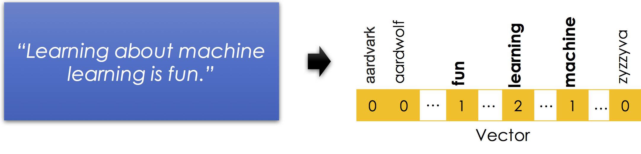
Notice
- Stop words are removed. Stop-words are words like
isandaboutthat in isolation contain very little information about the meaning of the sentence. Here is a good list of stop-words in many languages. - Word order information is lost. Nonetheless the vector still suggests that the sentence is about
fun,machines, andlearning. Thought there are many possible meanings learning machines have fun learning or learning about machines is fun learning ... - Capitalization and punctuation are typically removed.
- Sparse Encoding: is necessary to represent the bag-of-words efficiently. There are millions of possible words (including terminology, names, and misspellings) and so instantiating a
0for every word that is not in each record would be incredibly inefficient.
Why is it called a bag-of-words? A bag is another term for a multiset: an unordered collection which may contain multiple instances of each element.
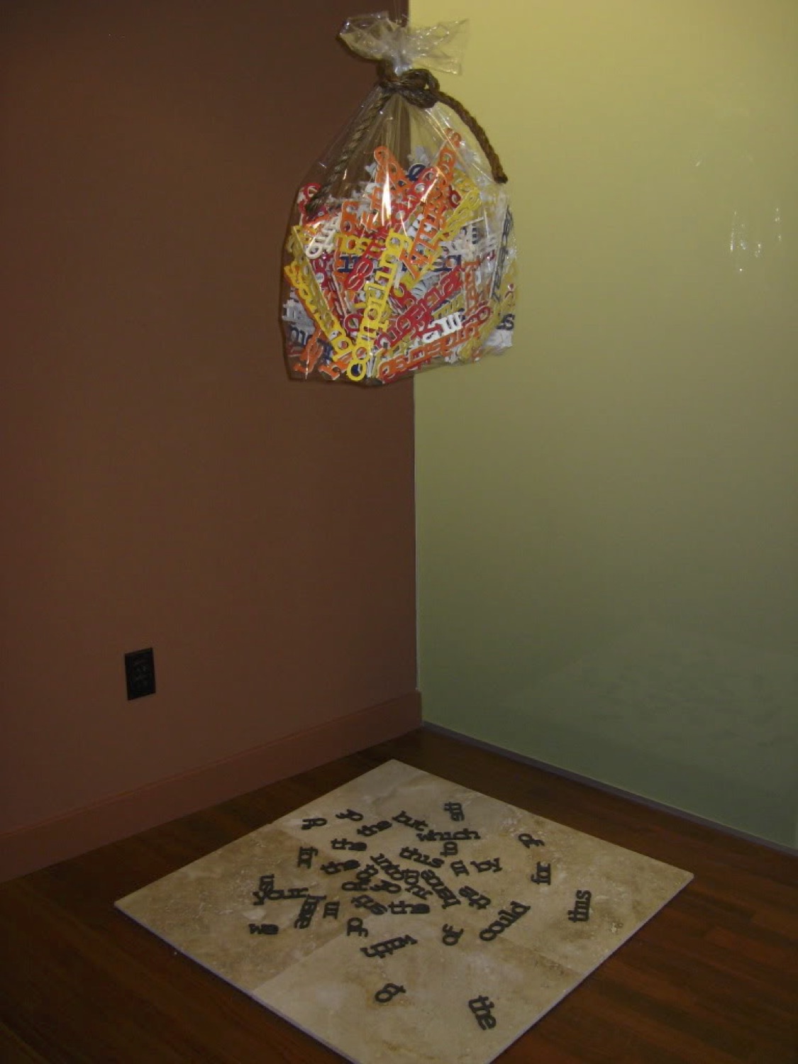
Professor Gonzalez is an "artist"
When professor Gonzalez was a graduate student at Carnegie Mellon University, he and several other computer scientists created the following art piece on display in the Gates Center:
Is this art or science?
Notice
- The unordered collection of words in the bag.
- The stop words on the floor.
- The missing broom. The original sculpture had a broom attached but the janitor got confused ....
Implementing the Bag-of-words Model
We can use sklearn to construct a bag-of-words representation of text
frost_text = [x for x in """
Some say the world will end in fire,
Some say in ice.
From what Ive tasted of desire
I hold with those who favor fire.
""".split("\n") if len(x) > 0]

frost_text
from sklearn.feature_extraction.text import CountVectorizer

# Construct the tokenizer with English stop words
bow = CountVectorizer(stop_words="english")

# fit the model to the passage
bow.fit(frost_text)
# Print the words that are kept
print("Words:", list(enumerate(bow.get_feature_names())))
print("Sentence Encoding: \n")
# Print the encoding of each line
for (s, r) in zip(frost_text, bow.transform(frost_text)):
    print(s)
    print(r)
    print("------------------")
The N-Gram Encoding
The N-Gram encoding is a generalization of the bag-of-words encoding designed to capture limited ordering information. Consider the following passage of text:
The book was not well written but I did enjoy it.
If we re-arrange the words we can also write:
The book was well written but I did not enjoy it.
Moreover, local word order can be important when making decisions about text. The n-gram encoding captures local word order by defining counts over sliding windows. In the following example a bi-gram ($n=2$) encoding is constructed:
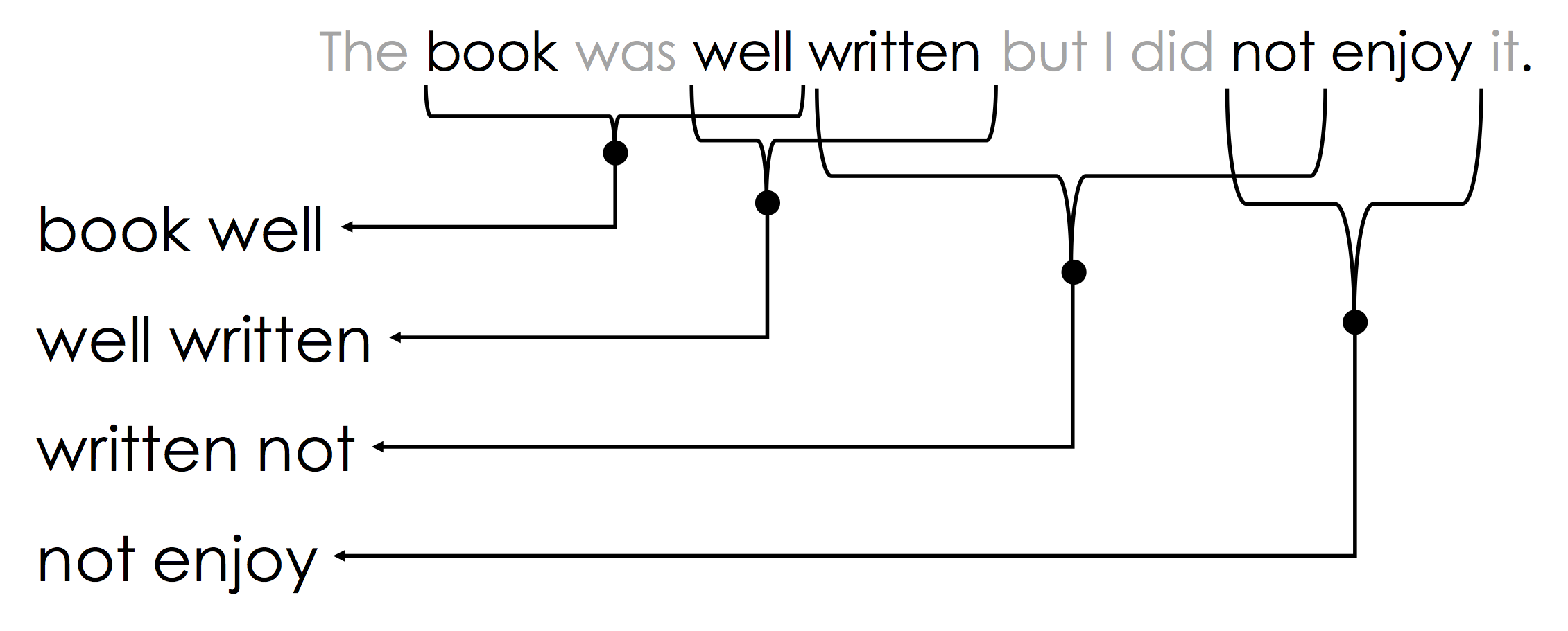
The above n-gram would be encoded in the sparse vector:
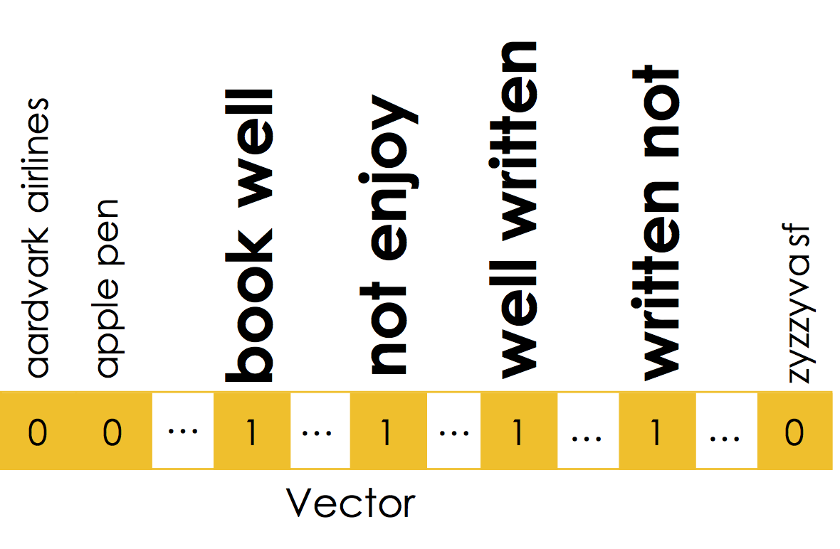
Notice that the n-gram captures key pieces of sentiment information: "well written" and "not enjoy".
N-grams are often used for other types of sequence data beyond text. For example, n-grams can be used to encode genomic data, protein sequences, and click logs.
N-Gram Issues
- The n-gram representation is hyper sparse and maintaining the dictionary of possible n-grams can be very costly. The hashing trick is a popular solution to approximate the sparse n-gram encoding. In the hashing trick each n-gram is mapped to a relatively large (e.g., 32bit) hash-id and the counts are associated with the hash index without saving the n-gram text in a dictionary. As a consequence, multiple n-grams are treated as the same.
- As $N$ increase the chance of seeing the same n-grams at prediction time decreases rapidly.
# Construct the tokenizer with English stop words
bigram = CountVectorizer(ngram_range=(1, 2))
# fit the model to the passage
bigram.fit(frost_text)
# Print the words that are kept
print("\nWords:",
      list(zip(range(0,len(bigram.get_feature_names())), bigram.get_feature_names())))
print("\nSentence Encoding: \n")
# Print the encoding of each line
for (s, r) in zip(frost_text, bigram.transform(frost_text)):
    print(s)
    print(r)
    print("------------------")