import numpy as np
import pandas as pd
import plotly.offline as py
import plotly.express as px
import plotly.graph_objects as go
from plotly.subplots import make_subplots
import cufflinks as cf
cf.set_config_file(offline=True, sharing=False, theme='solar')
Creating Synthetic Data
For this lecture we use a simple synthetic dataset to simplify the presentation of ideas.
n = 100
np.random.seed(42)
noise = 0.7
w_true = np.array([1., 3.])
quad = -4

x = np.sort(np.random.rand(n)*2 - 1.)
y = w_true[0] + w_true[1] * x + quad*(x**2) + noise * np.random.randn(n)
x[0] = -1.5
y[0] = 10
raw_data_plot = go.Scatter(x=x, y=y, name="Raw Data", mode='markers')
fig = go.Figure([raw_data_plot])
fig.update_layout(height=600)
Defining The Model and Loss Functions
Starting with a simple linear model:
def model(w, x):
    return w[0] + w[1] * x
From the previous lecture we showed how to analytically derive the minimizer for the squared loss:
def standard_units(x):
    return (x - np.mean(x)) / np.std(x)

def correlation(x, y):
    return np.mean (standard_units(x) * standard_units(y))

def slope(x, y):
    return correlation(x, y) * np.std(y) / np.std(x)

def intercept(x, y):
    return np.mean(y) - slope(x, y)*np.mean(x)
Computing the weights based on the functions from prior lecture.
w_mse = np.array([intercept(x,y), slope(x,y)])
w_mse
y_hat = model(w_mse, x)
analytic_mse_line = go.Scatter(x=x,y=y_hat, name="Analytic MSE")
fig = go.Figure([raw_data_plot, analytic_mse_line])
fig.update_layout(height=700)
fig
Visualizing the Residuals
The following code is for Plotly only to generate residual plots.
def residual_lines(x, y, yhat):
    return [
        go.Scatter(x=[x,x], y=[y,yhat],
               mode='lines', showlegend=False,
               line=dict(color='black', width = 0.5))
        for (x, y, yhat) in zip(x, y, y_hat)
    ]
fig = make_subplots(rows=2, cols=1, shared_xaxes=True)
for t in residual_lines(x,y,y_hat) + [raw_data_plot, analytic_mse_line]:
    fig.add_trace(t, row=1,col=1)
fig.add_trace(go.Scatter(x=x, y =   y -y_hat , mode='markers', name='Residuals'), row=2, col=1)
fig.add_trace(go.Scatter(x=[x.min(), x.max()], y = [0,0], showlegend=False), row=2, col=1)
fig.update_yaxes(title_text="Y", row=1, col=1)
fig.update_yaxes(title_text="Residual", row=2, col=1)
fig.update_layout(height=700)
Visualizing the Loss Surface
def mse_loss(yhat, y):
    return ((yhat - y)**2).mean()
Exhaustively try a large number of possible parameter values.
# Compute Range of intercpet values
w0values = np.linspace(w_mse[0]-1, w_mse[0]+1, 50)
# Compute Range of Slope values
w1values = np.linspace(w_mse[1]-1, w_mse[1]+1, 50)
# Construct "outer product of all possible values"
(u,v) = np.meshgrid(w0values, w1values)
# Convert into a tall matrix with each row corresponding to a possible parameterization
ws = np.vstack((u.flatten(),v.flatten())).transpose()
# Compute the Loss for each parameterization
mse_loss_values = np.array([mse_loss(y, model(w, x)) for w in ws]).reshape(u.shape)
Make a really cool looking visualization of the loss surface.
fig = make_subplots(rows=1, cols=2,
                    specs=[[{'type': 'contour'}, {'type': 'surface'}]])
# Make Contour Plot and Point
fig.add_trace(go.Contour(x=w0values, y=w1values, z=mse_loss_values , colorbar=dict(x=-.1)), row=1, col=1)
fig.add_trace(go.Scatter(x=[w_mse[0]], y=[w_mse[1]]), row=1, col=1)
# Make Surface Plot and Point
fig.add_trace(go.Surface(x=w0values, y=w1values, z=mse_loss_values, opacity=0.9), row=1, col=2)
fig.add_trace(go.Scatter3d(x=[w_mse[0]], y=[w_mse[1]], z=[mse_loss(y, model(w_mse,x))]), row=1, col=2)
# Cleanup Legend
fig.update_layout(scene=dict(xaxis=dict(title='Slope'), yaxis=dict(title='Intercept'), zaxis=dict(title="MSE Loss")))
fig.update_xaxes(title_text="Intercept", row=1, col=1)
fig.update_yaxes(title_text="Slope", row=1, col=1)
fig.update_layout(height=700)
Examining the $L^1$ Loss
We just solved the model for the $L^2$ loss. We now examine the $L^1$ loss. We first begin by visualizing the loss surface.
def abs_loss(yhat, y):
    return (np.abs(yhat - y)).mean()
# Compute Range of intercpet values
w0values = np.linspace(w_mse[0]-1, w_mse[0]+1, 50)
# Compute Range of Slope values
w1values = np.linspace(w_mse[1]-1, w_mse[1]+1, 50)
# Construct "outer product of all possible values"
(u,v) = np.meshgrid(w0values, w1values)
# Convert into a tall matrix with each row corresponding to a possible parameterization
ws = np.vstack((u.flatten(),v.flatten())).transpose()
# Compute the Loss for each parameterization
abs_loss_values = np.array([abs_loss(y, model(w, x)) for w in ws]).reshape(u.shape)
fig = make_subplots(rows=1, cols=2,
                    specs=[[{'type': 'contour'}, {'type': 'surface'}]])
# Make Contour Plot and Point
fig.add_trace(go.Contour(x=w0values, y=w1values, z=abs_loss_values, colorbar=dict(x=-.1)), row=1, col=1)
fig.add_trace(go.Scatter(x=[w_mse[0]], y=[w_mse[1]]), row=1, col=1)
# Make Surface Plot and Point
fig.add_trace(go.Surface(x=w0values, y=w1values, z=abs_loss_values, opacity=0.9), row=1, col=2)
fig.add_trace(go.Scatter3d(x=[w_mse[0]], y=[w_mse[1]], z=[abs_loss(y, model(w_mse,x))]), row=1, col=2)
# Cleanup Legend
fig.update_layout(scene=dict(xaxis=dict(title='Slope'), yaxis=dict(title='Intercept'), zaxis=dict(title="MSE Loss")))
fig.update_xaxes(title_text="Intercept", row=1, col=1)
fig.update_yaxes(title_text="Slope", row=1, col=1)
fig.update_layout(height=700)
fig = go.Figure([raw_data_plot, analytic_mse_line])
fig.update_layout(height=700)
fig
Quick Introduction to Algorithmic Differentiation
In this lecture we are going to introduce PyTorch. PyTorch is sort of like learning how to use Thor's hammer, it is way overkill for basically everything you will do and is probably the wrong solution to most problems you will encounter. However, it also really powerful and will give you the skills needed to take on very challenging problems.
import torch
Defining a variable $\theta$ with an initial value 1.0
theta = torch.tensor([1.0], requires_grad=True, dtype=torch.float64)
theta
Suppose we compute the following value from our tensor theta
z = (1 - torch.log(1 + torch.exp(theta)))**2
z
Notice that every derived value has an attached a gradient function that is used to compute the backwards path.
z.grad_fn
z.grad_fn.next_functions
z.grad_fn.next_functions[0][0].next_functions
We can visualize these functions
# !pip install torchviz
# !brew install graphviz
# from torchviz import make_dot
# make_dot(z)
If you were unable to run the above cell here is what the output looks like:
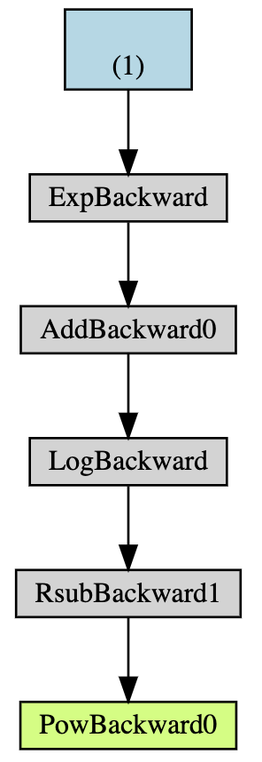
These backward functions tell Torch how to compute the gradient via the chain rule. This is done by invoking backward on the computed value.
z.backward()
theta.grad
We can use item to extract a single value.
theta.grad.item()
We can compare this witht he hand computed derivative:
\begin{align} \frac{\partial z}{\partial\theta} &= \frac{\partial}{\partial\theta}\left(1 - \log\left(1 + \exp(\theta)\right)\right)^2 \\ & = 2\left(1 - \log\left(1 + \exp(\theta)\right)\right)\frac{\partial}{\partial\theta} \left(1 - \log\left(1 + \exp(\theta)\right)\right)\\ & = 2\left(1 - \log\left(1 + \exp(\theta)\right)\right) (-1) \frac{\partial}{\partial\theta} \log\left(1 + \exp(\theta)\right) \\ & = 2\left(1 - \log\left(1 + \exp(\theta)\right)\right) \frac{-1}{1 + \exp(\theta)}\frac{\partial}{\partial\theta}\left(1 + \exp(\theta)\right) \\ & = 2\left(1 - \log\left(1 + \exp(\theta)\right)\right) \frac{-1}{1 + \exp(\theta)}\exp(\theta) \\ & = -2\left(1 - \log\left(1 + \exp(\theta)\right)\right) \frac{\exp(\theta)}{1 + \exp(\theta)} \end{align}def z_derivative(theta):
return -2 * (1 - np.log(1 + np.exp(theta))) * np.exp(theta) / (1. + np.exp(theta))
z_derivative(1.)
Minimizing the Absolute Loss Using Gradient Descent
Here we will use pytorch to implement gradient descent.
import torch
Converting numpy data to tensors. I will call them tx and ty to reduce confusion.
tx = torch.from_numpy(x)
ty = torch.from_numpy(y)
Defining a Model
The following defines a simple linear model as a basic class. The init function initializes the weights of the model. Here we have two weights, intercept and slope. The weights are initialized with requires_grad set to true so PyTorch will track the gradients of these weights.
The predict function makes a prediction based on the input x and the weights. In general, x will contain one or more inputs and so the function should work in either case.
the __call__ function allows me to call model.predict(x) as model(x) treating my models as a function.
class SimpleLinearModel:
    def __init__(self):
        self.w = torch.zeros(2, 1, requires_grad=True)

    def predict(self, x):
        w = self.w
        return w[0] + w[1] * x

    def __call__(self, x):
        return self.predict(x)
model = SimpleLinearModel()
model(tx)
The PyTorch nn.Module
The ideal way to define a model in pytorch is to extend the nn.Module class and introduce Parameters.
from torch import nn
class SimpleLinearModel(nn.Module):
    def __init__(self, w=None):
        super().__init__()
        # Creating a nn.Parameter object allows torch to track parameters for us
        if w is not None:
            self.w = nn.Parameter(torch.from_numpy(w))
        else:
            self.w = nn.Parameter(torch.zeros(2,1))
    def forward(self, x):
        w = self.w
        return w[0] + w[1] * x
    def numpy_parameters(self):
        """Return a numpy version of the parameters."""
        return np.array([p.detach().numpy() for p in self.parameters()]).flatten()
lin_model = SimpleLinearModel()
lin_model(tx)
The nn.Module class has some nice helper functions. For example, any parameters members of a module are automatically captured. This will be useful when we design modules with many parameters.
for p in lin_model.parameters():
    print(p)
We also added the numpy_parameters method to construct a single parameter numpy vector for visualization purposes.
lin_model.numpy_parameters()
Computing the Loss
There are many built in loss functions but we will build our own to see how it all works.
def abs_loss_torch(ypred, y):
    return torch.abs(ypred - y).mean()
loss = abs_loss_torch(lin_model(tx), ty)
loss
The item method returns the actual value from a single value tensor.
loss.item()
loss.backward()
lin_model.w.grad
# [p.grad for p in lin_model.parameters()]
# lin_model.w.grad.zero_() # <- this also works
lin_model.zero_grad()
[p.grad for p in lin_model.parameters()]
There is also a library of many loss functions in PyTorch
import torch.nn.functional as F
loss = F.l1_loss(lin_model(tx), ty)
loss.item()
Implementing Basic Gradient Descent
The following function implements a basic version of gradient descent.
def gradient_descent(model, loss_fn, x, y, lr=1., nsteps=100):
    values = [model.numpy_parameters()] # Track parameter values for later viz.
    for i in range(nsteps):
        loss = loss_fn(model(x), y)
        loss.backward()
        # We compute the update in a torch.no_grad context to prevent torch from
        # trying to compute the gradient of the gradient calculation.
        with torch.no_grad():
            for p in model.parameters():
                p -= lr / (i + 1) * p.grad
            # We also need to clear the gradient buffer otherwise future calls will
            # accumulate the gradient.
            model.zero_grad()
            # print(i, loss.item())
            values.append(model.numpy_parameters())
    return np.array(values)
lin_model = SimpleLinearModel()
values = gradient_descent(lin_model, F.l1_loss, tx, ty, nsteps=50, lr=6)
print("Loss =", F.l1_loss(ty, lin_model(tx)).item())
w_abs = lin_model.numpy_parameters()
print("[intecept, slope] =", w_abs)
w0values = np.linspace(-1., 1, 50)
w1values = np.linspace(-.5, 5, 50)
(u,v) = np.meshgrid(w0values, w1values)
ws = np.vstack((u.flatten(),v.flatten())).transpose()
loss = np.array([
    F.l1_loss(ty, SimpleLinearModel(w)(tx)).item() for w in ws]).reshape(u.shape)

fig = go.Figure([go.Contour(x=w0values, y=w1values, z=loss, colorbar=dict(x=-.2)),
          go.Scatter(x=[w_mse[0]], y=[w_mse[1]], name="MSE", mode="markers"),
          go.Scatter(x=[w_abs[0]], y=[w_abs[1]], name="Abs", mode="markers"),
          go.Scatter(x=values[:,0], y=values[:,1], name="Path", mode="markers+lines",
                     line=go.scatter.Line(color='white'))])
fig.update_layout(height=600, xaxis_title="Intercept", yaxis_title="Slope")
Visualizing the current best fit line
y_hat = lin_model(tx).detach().numpy()
gd_abs_line = go.Scatter(x=x,y=y_hat, name="GD ABS")
fig = make_subplots(rows=2, cols=1, shared_xaxes=True)
for t in residual_lines(x,y,y_hat) + [raw_data_plot, analytic_mse_line, gd_abs_line]:
    fig.add_trace(t, row=1,col=1)
fig.add_trace(go.Scatter(x=x, y = y - y_hat, mode='markers', name='Residuals'), row=2, col=1)
fig.add_trace(go.Scatter(x=[x.min(), x.max()], y = [0,0], showlegend=False), row=2, col=1)
fig.update_yaxes(title_text="Y", row=1, col=1)
fig.update_yaxes(title_text="Residual", row=2, col=1)
fig.update_layout(height=600)
Improving The Model
In the above we notice some curvature in the residual plot and decide to build a more complex model with an extra quadratic term.
class PolynomialModel(nn.Module):
    def __init__(self, w=None, p=2):
        super().__init__()
        # Creating a nn.Parameter object allows torch to track parameters for us
        if w is not None:
            self.w = nn.Parameter(torch.from_numpy(w))
        else:
            self.w = nn.Parameter(torch.zeros(p+1,1))
    def forward(self, x):
        w = self.w
        return torch.sum(torch.stack([w[i] * x ** i for i in range(len(w))]), dim=0)
    def numpy_parameters(self):
        """Return a numpy version of the parameters."""
        return np.array([p.detach().numpy() for p in self.parameters()]).flatten()
quad_model = PolynomialModel(np.array([1., 2., 3.]))
quad_model(tx)
quad_model = PolynomialModel()
values = gradient_descent(quad_model, F.l1_loss, tx, ty, nsteps=500, lr=10)
print("Loss =", F.l1_loss(ty, quad_model(tx)).item())
w_quad_abs = quad_model.numpy_parameters()
print("[intecept, slope, quad_term] =", w_quad_abs)
y_hat = quad_model(tx).detach().numpy().flatten()

gd_quad_abs_line = go.Scatter(x=x, y=y_hat, name="GD Quad ABS")
fig = make_subplots(rows=2, cols=1, shared_xaxes=True)
for t in residual_lines(x,y,y_hat) + [raw_data_plot, analytic_mse_line, gd_abs_line, gd_quad_abs_line]:
    fig.add_trace(t, row=1,col=1)
fig.add_trace(go.Scatter(x=x, y = y - y_hat , mode='markers', name='Residuals'), row=2, col=1)
fig.add_trace(go.Scatter(x=[x.min(), x.max()], y = [0,0], showlegend=False), row=2, col=1)
fig.update_yaxes(title_text="Y", row=1, col=1)
fig.update_yaxes(title_text="Residual", row=2, col=1)
fig.update_layout(height=600)
Implementing Stochastic Gradient Descent
First we need a mechanism to sample the data. Since this is central to SGD (and therefore PyTorch) there is a built in way to do this:
from torch.utils.data import TensorDataset, DataLoader
dataset = TensorDataset(tx, ty)
loader = DataLoader(dataset, batch_size=20, shuffle=True)
[dict(x=x, y=y) for x, y in loader]
Basic SGD implementation
def stochastic_gradient_descent(model, loss_fn, dataset, lr=1., nepochs=100, batch_size=10):
    loader = DataLoader(dataset, batch_size=batch_size, shuffle=True)
    values = [model.numpy_parameters()] # Track parameter values for later viz.
    for i in range(nepochs):
        for (x, y) in loader:
            loss = loss_fn(model(x), y)
            loss.backward()
            # We compute the update in a torch.no_grad context to prevent torch from
            # trying to compute the gradient of the gradient calculation.
            with torch.no_grad():
                for p in model.parameters():
                    p -= lr / (i + 1) * p.grad
                # We also need to clear the gradient buffer otherwise future calls will
                # accumulate the gradient.
                model.zero_grad()
                # print(i, loss.item())
                values.append(model.numpy_parameters())
    return np.array(values)
quad_model_sgd = PolynomialModel(p=2)
values = stochastic_gradient_descent(quad_model_sgd, F.l1_loss, dataset,
                                     lr=1.0, nepochs=20, batch_size=10)
print("Loss =", F.l1_loss(ty, quad_model_sgd(tx)).item())
w_quad_abs_sgd = quad_model_sgd.numpy_parameters()
print("[intecept, slope, quad_term] =", w_quad_abs_sgd)
fig = go.Figure([go.Scatter3d(x=values[:,0], y=values[:,1], z=values[:,2],
                              marker=dict(color=np.linspace(0,1,values.shape[0]))
                             )])
fig.update_layout(height = 800)
py.iplot(fig)
Improving SGD with better optimizers
from torch.optim import Adam, SGD
def adam_sgd(model, loss_fn, dataset, lr=.1, nepochs=100, batch_size=10):
    loader = DataLoader(dataset, batch_size=batch_size, shuffle=True)
    opt = Adam(model.parameters(), lr=lr)
    values = [model.numpy_parameters()] # Track parameter values for later viz.
    for i in range(nepochs):
        for (x, y) in loader:
            loss = loss_fn(model(x), y)
            loss.backward()
            opt.step()
            model.zero_grad()
            values.append(model.numpy_parameters())
    return np.array(values)
quad_model_sgd2 = PolynomialModel(p=2)
values = adam_sgd(quad_model_sgd2, F.l1_loss, dataset, lr = 0.1, nepochs=100, batch_size=10)
print("Loss =", F.l1_loss(ty, quad_model_sgd2(tx)).item())
w_quad_abs_sgd2 = quad_model_sgd2.numpy_parameters()
print("[intecept, slope, quad_term] =", w_quad_abs_sgd2)
More Advanced Model
poly_model_sgd = PolynomialModel(p=12)
values = adam_sgd(poly_model_sgd, F.l1_loss, dataset, lr=0.01, nepochs=500, batch_size=10)
print("Loss =", F.l1_loss(ty, poly_model_sgd(tx)).item())
Examining this Amazing Fit.
xtest = np.linspace(x.min(), x.max(), 1000)
y_hat = poly_model_sgd(torch.from_numpy(xtest)).detach().numpy().flatten()

poly_model_line = go.Scatter(x=xtest, y=y_hat, name="Poly Model Line")
fig = go.Figure([raw_data_plot, analytic_mse_line, gd_abs_line, gd_quad_abs_line, poly_model_line])
fig.update_yaxes(title_text="Y")
fig.update_layout(height=600)