import numpy as np
import pandas as pd

# Plotly plotting support
import plotly.plotly as py
# import plotly.offline as py
# py.init_notebook_mode()

# import cufflinks as cf
# cf.go_offline() # required to use plotly offline (no account required).

import plotly.graph_objs as go
import plotly.figure_factory as ff

# Make the notebook deterministic 
np.random.seed(42)

Cross Validation and the Bias Variance Tradeoff

This notebook which accompanies the lecture on the Bias Variance Tradeoff and Regularization.

Notebook created by Joseph E. Gonzalez for DS100.

Toy Dataset

As with the previous lectures we will continue to use an easy to visualize synthetic dataset.

np.random.seed(42)
n = 50
sigma = 10
X = np.linspace(-10, 10, n)
X = np.sort(X)
Y = 2. * X + 10. + sigma * np.random.randn(n) +  20*np.sin(X) + 0.8*(X)**2
X = X/5
data_points = go.Scatter(name="data", x=X, y=Y, mode='markers')
py.iplot([data_points])

Making a train Test Split

It is always a good habbit to split data into training and test sets.

from sklearn.model_selection import train_test_split 
X_tr, X_te, Y_tr, Y_te = train_test_split(X, Y, test_size=0.25, random_state=42)
train_points = go.Scatter(name="Train Data", 
                          x=X_tr, y=Y_tr, mode='markers',  marker=dict(color="blue", symbol="o"))
test_points = go.Scatter(name="Test Data",
                         x=X_te, y=Y_te, mode='markers', marker=dict(color="red", symbol="x"))
py.iplot([train_points, test_points])

Polynomial Features:

In the following we work through a basic bias variance tradeoff for different numbers of polynomial features. To make things a bit more interesting we will also add an additional sine feature:

$$ \large \Phi_d(x) = \left[\sin(\omega x), x, x^2, \ldots, x^d \right] $$

with the appropriate $\omega = 5$ value determined from prior knowledge (because we created the data).

We use the following Python function to generate a $\Phi$:

def poly_phi(k):
    return lambda X: np.array([np.sin(X*5)] + [X ** i for i in range(1, k+1)]).T

We will consider the following basis sizes:

basis_sizes = [1, 2, 5, 8, 16, 24, 32]

Create a $\Phi$ feature matrix for each number of basis:

Phis_tr = { k: poly_phi(k)(X_tr) for k in basis_sizes }

Train a model for each number of feature

from sklearn import linear_model
models = {}
for k in Phis_tr:
    model = linear_model.LinearRegression()
    model.fit(Phis_tr[k], Y_tr)
    models[k] = model

Visualize the various models

The following code is a bit complicated but essentially makes an interactive visualization of the various models.

# Make the x values where plot points will be generated
X_plt = np.linspace(np.min(X)-1, np.max(X)+1, 200)

# Generate the Plotly line objects by predicting the value at each X_plt
lines = []
for k in sorted(models.keys()):
    ytmp = models[k].predict(poly_phi(k)(X_plt))
    # Plotting software fails with large numbers
    ytmp[ytmp > 500] = 500
    ytmp[ytmp < -500] = -500
    lines.append(
        go.Scatter(name="degree "+ str(k), x=X_plt,
                   y = ytmp,visible=False))

# Construct steps for the interactive slider
lines[0].visible=True
steps = []
for i in range(len(lines)):
    step = dict(
        label = lines[i]['name'],
        method = 'restyle',
        args = ['visible', [False] * (len(lines)+1)],
    )
    step['args'][1][0] = True
    step['args'][1][i+1] = True # Toggle i'th trace to "visible"
    steps.append(step)

# Build the slider object
sliders = [dict(active = 0, pad = {"t": 20}, steps = steps)]

# render the plot
layout = go.Layout(xaxis=dict(range=[np.min(X_plt), np.max(X_plt)]), 
                   yaxis=dict(range=[np.min(Y) -5 , np.max(Y)+5]),
                   sliders=sliders)
py.iplot(go.Figure(data = [train_points] + lines, layout=layout), filename="poly_curve_comparison")

Cross Validation

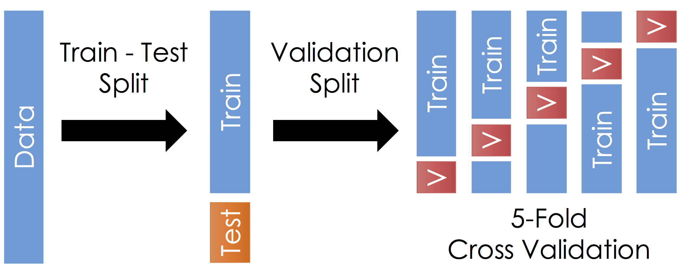
With the remaining training data:

1. Split the remaining training dataset k-ways as in the Figure above. The figure uses 5-Fold which is standard. You should split the data in the same way you constructed the test set (this is typically randomly)
2. For each split train the model on the training fraction and then compute the error (RMSE) on the validation fraction.
3. Average the error across each validation fraction to estimate the test error.

Define the error Function

We will continue to use the mean squared error but this time rather than define it ourselves we will import it from scikit-learn.

from sklearn.metrics import mean_squared_error

In the following we compute the cross validated RMSE for different numbers of polynomial basis values

from sklearn.model_selection import KFold
kfold_splits = 5
kfold = KFold(kfold_splits, shuffle=True, random_state=42)

mse_scores = []
poly_degrees = np.arange(1,16)
for k in poly_degrees:
    Phi = poly_phi(k)(X_tr)
    
    # One step in k-fold cross validation
    def score_model(train_index, test_index):
        model = linear_model.LinearRegression()
        model.fit(Phi[train_index,], Y_tr[train_index])
        return mean_squared_error(Y_tr[test_index], model.predict(Phi[test_index,]))
    

    score = np.mean([score_model(tr_ind, te_ind) 
                     for (tr_ind, te_ind) in kfold.split(Phi)])
    mse_scores.append(score)
    
    
rmse_scores = np.sqrt(np.array(mse_scores))

py.iplot(
    go.Figure(
        data=[go.Scatter(name="CV Curve", x=poly_degrees, y=rmse_scores),
              go.Scatter(name="Optimum", x=[poly_degrees[np.argmin(rmse_scores)]], y=[np.min(rmse_scores)],
                         mode="markers", marker=dict(color="red", size=10))
             ],
        layout=go.Layout(xaxis=dict(title="Degree"), yaxis=dict(title="CV RMSE"))),
    filename="basis_function_cv_curve")

---

Questions?

1. Is 2 a reasonable answer given the data? (Look at the earlier plot.)
2. Does this depend on the order in which we consider basis?

Variance

1. What happens if we repeat the training procedure with different versions of our trainin data?

2. How will the models change as we inrease the degree of our polynomial?

---

Here we use cross validation to simulate multiple train and test splits by splitting the training data into train and validation datasets. We then visualize each of the corresponding models.

from sklearn.model_selection import KFold

# Construct a KFold object which will define random index splits
kfold_splits = 5
kfold = KFold(kfold_splits, shuffle=True, random_state=42)

# Construct the lines
lines = []

# Make the test lines
X_plt = np.linspace(np.min(X)-1, np.max(X)+1, 200)

# for each train validation split (we ignore the validation data)
for k in basis_sizes:
    for (tr_ind, val_ind) in kfold.split(X_tr):
        # Construct the Phi matrices for each basis size
        Phi = poly_phi(k)(X_tr[tr_ind]) 
        # Fit the model
        model = linear_model.LinearRegression()
        model.fit(Phi, Y_tr[tr_ind])
        # Make predictions at the plotting points
        ytmp = model.predict(poly_phi(k)(X_plt))
        # Plotly has a bug and fails with large numbers
        ytmp[ytmp > 500] = 500
        ytmp[ytmp < -500] = -500
        line = go.Scatter(name="degree "+ str(k), visible=False,
                          x=X_plt, y=ytmp)
        lines.append(line)

for l in lines[0:kfold_splits]:
    l.visible=True

steps = []
for i in range(len(basis_sizes)):
    step = dict(
        label = "Degree " + str(basis_sizes[i]) ,
        method = 'restyle',
        args = ['visible', [False] * (len(lines)+1)]
    )
    step['args'][1][-1] = True
    for u in range(i*kfold_splits, (i+1)*kfold_splits):
        step['args'][1][u] = True # Toggle i'th trace to "visible"
    steps.append(step)
    
sliders = [dict(
    active = 0,
    pad = {"t": 20},
    steps = steps
)]

layout = go.Layout(xaxis=dict(range=[np.min(X_plt), np.max(X_plt)]), 
                   yaxis=dict(range=[np.min(Y) -5 , np.max(Y) + 5]),
                   sliders=sliders,
                   showlegend=False)

py.iplot(go.Figure(data = lines + [train_points], layout=layout), filename="cv_bv_slider")
    

Return to Slides!

---