Lecture 1 – Data 100, Fall 2020
by Anthony D. Joseph
adapted from Joey Gonzalez, Josh Hug, Suraj Rampure
import pandas as pd
import numpy as np
import matplotlib.pyplot as plt
import seaborn as sns

## Plotly plotting support
import plotly.offline as py
py.init_notebook_mode()
import plotly.graph_objs as go
import plotly.figure_factory as ff
import plotly.express as px
# import cufflinks as cf
# cf.set_config_file(offline=False, world_readable=False, theme='ggplot')
Load and clean the roster
names = pd.read_csv("names.csv")
major_year = pd.read_csv("major_year.csv")[['Majors', 'Terms in Attendance']]
names.head(20)
names['Name'] = names['Name'].str.lower()
print("Number of Students:", len(names))
names.head(20)
names.describe()
major_year["Majors"] = major_year["Majors"].str.replace("BS","").str.replace("BA","")
major_year['Terms in Attendance'] = major_year['Terms in Attendance'].astype(str)
major_year.head(20)
major_year.describe()
We now know the general structure of our datasets. Let's now ask some questions.
What is the distribution of the lengths of students' names in this class?
sns.distplot(names['Name'].str.len(), rug=True, axlabel="Number of Characters");

What are the majors of students in the class?
(
    major_year["Majors"]
        .str.lower()
        .value_counts().sort_values(ascending=False)
        .head(20).plot(kind='barh', title = "Major")
);

px.bar(major_year['Majors'].value_counts().to_frame().reset_index().head(20),
       x = 'Majors',
       y = 'index',
       orientation = 'h')
What is the gender of the class?
How can we answer this question?
print(major_year.columns)
print(names.columns)
Ideas:
- What do we mean by gender?
- Can we use the name to estimate gender?
- How would we build model of gender given the name?
- Where can we get data for such a model?
US Social Security Data
Public dataset containing baby names and their sex.
Understanding the Setting
In Data 100 you will have to learn about different data sources on your own.
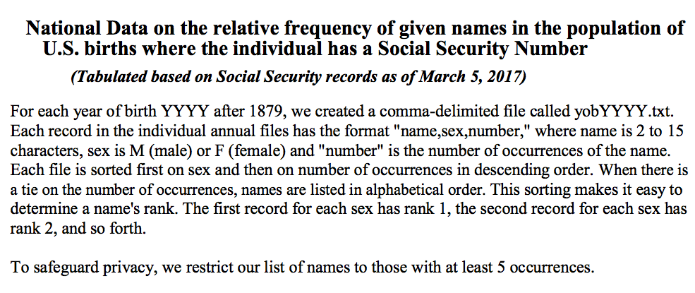
Reading from SSN Office description:
All names are from Social Security card applications for births that occurred in the United States after 1879. Note that many people born before 1937 never applied for a Social Security card, so their names are not included in our data. For others who did apply, our records may not show the place of birth, and again their names are not included in our data.
All data are from a 100% sample of our records on Social Security card applications as of March 2017.
Get data programatically
import urllib.request
import os.path

# Download data from the web directly
data_url = "https://www.ssa.gov/oact/babynames/names.zip"
local_filename = "babynames.zip"
if not os.path.exists(local_filename): # if the data exists don't download again
    with urllib.request.urlopen(data_url) as resp, open(local_filename, 'wb') as f:
        f.write(resp.read())


# Load data without unzipping the file
import zipfile
babynames = []
with zipfile.ZipFile(local_filename, "r") as zf:
    data_files = [f for f in zf.filelist if f.filename[-3:] == "txt"]
    def extract_year_from_filename(fn):
        return int(fn[3:7])
    for f in data_files:
        year = extract_year_from_filename(f.filename)
        with zf.open(f) as fp:
            df = pd.read_csv(fp, names=["Name", "Sex", "Count"])
            df["Year"] = year
            babynames.append(df)
babynames = pd.concat(babynames)


babynames.head()
A little bit of data cleaning:
babynames['Name'] = babynames['Name'].str.lower()
babynames.tail()
Exploratory Data Analysis
How many people does this data represent?
format(babynames['Count'].sum(), ',d')
len(babynames)
Is this number low or high?
It seems low. However the social security website states:
All names are from Social Security card applications for births that occurred in the United States after 1879. **Note that many people born before 1937 never applied for a Social Security card, so their names are not included in our data.** For others who did apply, our records may not show the place of birth, and again their names are not included in our data. All data are from a 100% sample of our records on Social Security card applications as of the end of February 2016.Let's query to find rows that match desired conditions.
babynames[(babynames['Name'] == 'vela') & (babynames['Sex'] == 'F')].tail(5)
babynames[(babynames['Name'] == 'anthony') & (babynames['Year'] == 2000)]
babynames.query('Name.str.contains("data")', engine='python')
Proportion of Male and Female Individuals Over Time
In this example we construct a pivot table which aggregates the number of babies registered for each year by Sex.
pivot_year_name_count = pd.pivot_table(babynames,
        index=['Year'], # the row index
        columns=['Sex'], # the column values
        values='Count', # the field(s) to processed in each group
        aggfunc=np.sum,
    )

pivot_year_name_count.head()
pivot_year_name_count.plot(title='Names Registered that Year');

fig = go.Figure()
fig.add_trace(go.Scatter(x = pivot_year_name_count.index, y = pivot_year_name_count['F'], name = 'F', line=dict(color='gold')))
fig.add_trace(go.Scatter(x = pivot_year_name_count.index, y = pivot_year_name_count['M'], name = 'M', line=dict(color='blue')))
fig.update_layout(xaxis_title = 'Year', yaxis_title = 'Names Registered')
How many unique names for each year?
pivot_year_name_nunique = pd.pivot_table(babynames,
        index=['Year'],
        columns=['Sex'],
        values='Name',
        aggfunc=lambda x: len(np.unique(x)),
    )

pivot_year_name_nunique.plot(
   title='Number of Unique Names');

Some observations:
- Registration data seems limited in the early 1900s. Because many people did not register before 1937.
- You can see the baby boomers and the echo boom.
- Females have greater diversity of names.
Computing the Proportion of Female Babies For Each Name
sex_counts = pd.pivot_table(babynames, index='Name', columns='Sex', values='Count',
                            aggfunc='sum', fill_value=0., margins=True)
sex_counts.head()
Compute proportion of female babies given each name.
prop_female = sex_counts['F'] / sex_counts['All']
prop_female.head(10)
prop_female.tail(10)
Testing a few names
prop_female['audi']
prop_female['anthony']
prop_female['joey']
prop_female['avery']
prop_female["sarah"]
prop_female["min"]
prop_female["pat"]
Build Simple Classifier (Model)
We can define a function to return the most likely Sex for a name. If there is an exact tie, the function returns Male. If the name does not appear in the social security dataset, we return Unknown.
def sex_from_name(name):
    lower_name = name.lower()
    if lower_name in prop_female.index:
        return 'F' if prop_female[lower_name] > 0.5 else 'M'
    else:
        return "Unknown"
sex_from_name("audi")
sex_from_name("joey")
What fraction of students in Data 100 this semester have names in the SSN dataset?
student_names = pd.Index(names["Name"]).intersection(prop_female.index)
print("Fraction of names in the babynames data:" , len(student_names) / len(names))
Which names are not in the dataset?
Why might these names not appear?
missing_names = pd.Index(names["Name"]).difference(prop_female.index)
missing_names
Estimating the fraction of female and male students
names['Pred. Sex'] = names['Name'].apply(sex_from_name)
(names[names['Pred. Sex'] != "Unknown"]['Pred. Sex'].value_counts()/len(names[names['Pred. Sex'] != "Unknown"])).plot(kind="barh");

Using simulation to estimate uncertainty
Previously we treated a name which is given to females 40% of the time as a "Male" name. This doesn't capture our uncertainty. We can use simulation to provide a better distributional estimate.
Restricting our attention to students in the class
len(prop_female)
ds100_prob_female = prop_female.loc[prop_female.index.intersection(names['Name'])]
ds100_prob_female.tail(20)
Running the simulation
one_simulation = np.random.rand(len(ds100_prob_female)) < ds100_prob_female
one_simulation.tail(20)
# function that performs many simulations
def simulate_class(students):
    is_female = np.random.rand(len(ds100_prob_female)) < ds100_prob_female
    return np.mean(is_female)

fraction_female_simulations = np.array([simulate_class(names) for n in range(10000)])
# plt.hist(fraction_female_simulations, bins=np.arange(0.4, 0.46, 0.0025), ec='w');
# pd.Series(fraction_female_simulations).iplot(kind="hist", bins=30)
ff.create_distplot([fraction_female_simulations], ['Fraction Female'], bin_size=0.0025, show_rug=False)