# Standard imports
import matplotlib.pyplot as plt
%matplotlib inline
import seaborn as sns
sns.set_context("talk")
Numpy Review
This is a brief overview of numpy for DS100. The Jupyter Notebook can be obtained here: Numpy_Review.ipynb.
Importing Numpy
It is customary to import Numpy as np:
import numpy as np
As you learned in homework one the np.array is the key data structure in numpy for dense arrays of data.
Creating Arrays
You can build arrays from python lists.
Data 8 Compatibility: In data8 you used a datascience package function called make_array which wraps the more standard np.array function we will use in this class.
np.array([[1.,2.], [3.,4.]])
np.array([x for x in range(5)])
Array's don't have to contain numbers:
np.array([["A", "matrix"], ["of", "words."]])
Making Arrays of Zeros
np.zeros(5)
Making Arrays of Ones
np.ones([3,2])
np.eye(4)
Making Arrays from ranges:
The np.arange(start, stop, step) function is like the python range function.
np.arange(0, 10, 2)
You can make a range of other types as well:
np.arange(np.datetime64('2016-12-31'), np.datetime64('2017-02-01'))
Interpolating numbers
The linspace(start,end,num) function generates num numbers evenly spaced between the start and end.
np.linspace(0, 5, 10)
Learn more about working with datetime objects.
A random array
You can also generate arrays of random numbers (we will cover this in greater detail later).
randngenerates random numbers from a Normal(mean=0, var=1) distribution.randgenerates random numbers from a Uniform(low=0, high=1) distribution.permutationgenerates a random permutation of a sequence of numbers.
np.random.randn(3,2)
np.random.rand(3,2)
np.random.permutation(range(0,10))
Properties of Arrays
Shape
Arrays have a shape which corresponds to the number of rows, columns, fibers, ...
A = np.array([[1., 2., 3.], [4., 5., 6.]])
print(A)
A.shape
Type
Arrays have a type which corresponds to the type of data they contain
A.dtype
np.arange(1,5).dtype
(np.array([True, False])).dtype
np.array(["Hello", "Worlddddd!"]).dtype
What does <U6 mean?
<Little EndianUUnicode6length of longest string
and we can change the type of an array:
np.array([1,2,3]).astype(float)
np.array(["1","2","3"]).astype(int)
Learn more about numpy array types
Polymorphism
Can an array have more than one type?
np.array([1,2,3, "cat", True])
Does the following command work:
x = np.array([1,2,3,4])
x[3] = "cat"
x = np.array([1,2,3,4])
# x[3] = "cat" # <-- uncomment this line to find out
Jagged Arrays
Is the following valid?
A = np.array([[1, 2, 3], [4, 5], [6]])
A = np.array([[1, 2, 3], [4, 5], [6]])
A
What happened?
A.shape
print(A.dtype)
print(A[0])
print(A[1])
print(A[2])
Issues with Jagged Arrays

Jagged arrays can be problematic:
- Difficult to index (extract columns).
A[0,1]
> Error
A[0][1]
> 2
- Not as efficiently represented in contiguous memory.
Reshaping
Often you will need to reshape matrices. Suppose you have the following array:
np.arange(1,13)
What will the following produce:
np.arange(1,13).reshape(4,3)
Option A:
array([[ 1,  2,  3],
       [ 4,  5,  6],
       [ 7,  8,  9],
       [10, 11, 12]])
Option B:
array([[ 1,  5,  9],
       [ 2,  6, 10],
       [ 3,  7, 11],
       [ 4,  8, 12]])
Solution
A = np.arange(1,13).reshape(4,3)
A
Flatting Matrix
Flattening a matrix (higher dimensional array) produces a one dimensional array.
A.flatten()
Advanced: Array representation
Numpy stores data contiguously in memory
print(A.dtype)
A.data.tobytes()
Numpy stores matrices in row-major order (by rows)
print(np.arange(1,13).reshape(4,3, order='C'))
print()
print(np.arange(1,13).reshape(4,3, order='F'))
What does the 'F' mean?
Fortran ordering. In BLAS libraries are specified for Fortran and C programming languages which differ both in the column (Fortran) or row (C) indexing.
Slicing
From homework 1 you should already be pretty good at Slicing so let's test your slicing knowledge.

- Program 1:
x[:, 0]
**Answer**
B
- Program 2:
x[0, :]
**Answer**
A
- Program 3:
x[:2, 1:]
**Answer**
H
- Program 4:
x[0::2, :]
**Answer**
D
Understanding the slice syntax
begin:end:stride
Modifying a Slice
Suppose I wanted to make all entries in my matrix 0 in the top right corner as in (H) above.
H = np.arange(1,13).reshape(4,3)
print("Before:\n", H)
H[:2, 1:] = 0
print("After:\n", H)
Boolean Indexing
We can apply boolean operations to arrays. This is essential when trying to select and modify individual elements.
Question: Given the following definition of A:
[[   1.    2.    3.]
 [   4.    5. -999.]
 [   7.    8.    9.]
 [  10. -999. -999.]]
what will the following output:
A > 3
- Option A:
False
- Option B:
array([[False, False, False],
       [ True,  True, False],
       [ True,  True,  True],
       [ True, False, False]], dtype=bool)
A = np.array([[  1.,   2.,   3.],
       [  4.,   5.,   -999.0],
       [  7.,   8.,   9.],
       [ 10.,  -999.0,  -999.0]])

A > 3.
Question: What will the following output
A = np.array([[   1.,    2.,    3.],
       [   4.,    5., -999.],
       [   7.,    8.,    9.],
       [  10., -999., -999.]])

A[A > 3]
- Option A:
array([ 4, 7, 10, 5, 8, 11, 6, 9, 12])
- Option B:
array([ 4., 5., 7., 8., 9., 10.])
- Option C:
array([[  nan,   nan,  nan],
       [  4.,    5.,   nan],
       [  7.,    8.,   9.],
       [ 10.,    nan,  nan]])
A = np.array([[  1.,   2.,   3.],
       [  4.,   5.,   -999.0],
       [  7.,   8.,   9.],
       [ 10.,  -999.0,  -999.0]])

A[A > 3]
Question: Replace the -999.0 entries with np.nan.
array([[   1.,    2.,    3.],
       [   4.,    5., -999.],
       [   7.,    8.,    9.],
       [  10., -999., -999.]])
Solution
A = np.array([[  1.,   2.,   3.],
       [  4.,   5.,   -999.0],
       [  7.,   8.,   9.],
       [ 10.,  -999.0,  -999.0]])
- Construct a boolean array that indicates where the value is 999.0:
ind = (A == -999.0)
print(ind)
- Assign
np.nanto all theTrueentires:
A[ind] = np.nan
A
Question: What might -999.0 represent? Why might I want to replace the -999.0 with a np.nan?
Solution: It could be safer in calculations. For example when computing the mean of the transformed A we get:
print(A)
np.mean(A)
Perhaps instead we want:
np.nanmean(A)
help(np.nanmean)
More Complex Bit Logic
Often we will want to work with multiple different arrays at once and select subsets of entries from each array. Consider the following example:
names = np.array(["Joey", "Henry", "Joseph",
                  "Jim", "Sam", "Deb", "Mike",
                  "Bin", "Joe", "Andrew", "Bob"])

favorite_number = np.arange(len(names))
Suppose a subset of these people are staff members:
staff = ["Joey", "Deb", "Sam"]
Question:
How could we compute the sum of the staff members favorite numbers?
One solution is to use for loops:
total = 0
for i in range(len(names)):
    if names[i] in staff:
        total += favorite_number[i]

print("total:", total)
Another solution would be to use the np.in1d function to determine which people are staff.
is_staff = np.in1d(names, staff)
is_staff
Boolean indexing
favorite_number[is_staff].sum()
Question:
What does the following expression compute:
starts_with_j = np.char.startswith(names, "J")
starts_with_j[is_staff].mean()
The fraction of the staff have names that begin with J?
starts_with_j = np.char.startswith(names, "J")
starts_with_j[is_staff].mean()
Question:
What does it mean to take the mean of an array of booleans?
The values True and False correspond to the integers 1 and 0 and are treated as such in mathematical expressions (e.g., mean(), sum(), as well as linear algebraic operations).
Question
What does the following expression compute:
favorite_number[starts_with_j & is_staff].sum()
The sum of the favorite numbers of staff starting with J
favorite_number[starts_with_j & is_staff].sum()
A Note on using Array operations
data = np.random.rand(1000000)
%%timeit
s = 0
for x in data:
    if x > 0.5:
        s += x
result = s/len(data)
%%timeit
result = data[data > 0.5].mean()
Important Points
Using the array abstractions instead of looping can often be:
- Clearer
- Faster
These are fundamental goals of abstraction.
Numpy arrays support standard mathematical operations
A = np.arange(1., 13.).reshape(4,3)
print(A)
A * 0.5 + 3
notice that operations are element wise.
A.T
A.sum()
A.mean()
Be Careful with Floating Point Numbers
What is the value of the following: $$ A - \exp \left( \log \left( A \right) \right) $$
Solution:
A = np.arange(1., 13.).reshape(4,3)
print(A)

(A - np.exp(np.log(A)))
What happened?!
Floating point precision is not perfect and we are applying transcendental functions.
0.1 + 0.2 == 0.3
print(0.1 + 0.2)
For these situations consider using np.isclose:
help(np.isclose)
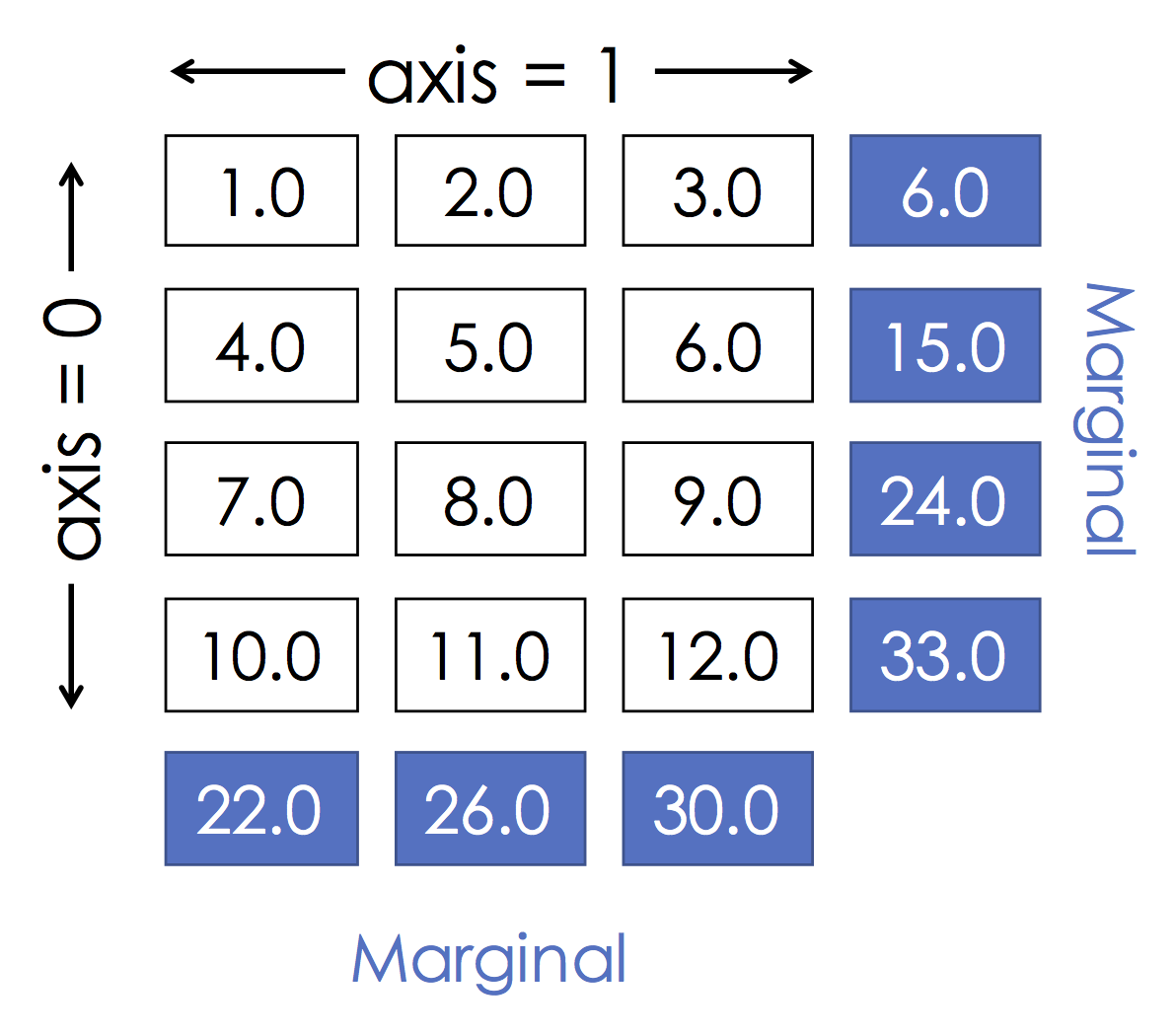
Grouping by row:
A.sum(axis=0)
This is the same as:
(nrow, ncols) = A.shape

s = np.zeros(ncols)

for i in range(nrows):
    s += A[i,:]

print(s)
Grouping by col:
A.sum(axis=1)
This is the same as:
(nrows, ncols) = A.shape

s = np.zeros(nrows)

for i in range(ncols):
    s += A[:,i]

print(s)
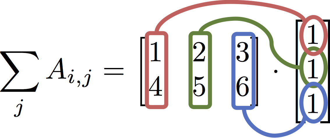
$$ \texttt{A.sum( axis = 1) } = \sum_j A_{i,j} = \begin{bmatrix} 1 & 2 & 3 \\ 4 & 5 & 6\end{bmatrix} \cdot \begin{bmatrix} 1 \\ 1 \\ 1\end{bmatrix} $$
A = np.array([[1, 2, 3], [4, 5, 6]])
b = np.ones(3)
A * b
Explanation:
We ended up computing an element-wise product. The vector of ones was replicated once for each row and then used to scale the entire row.
The correct expression for matrix multiplication
A.dot(b)
In the later python versions (>3.5) you can use the infix operator @ which is probably easier to read
A @ b
Suppose you are asked to solve the following system of linear equations:
$$ 5x - 3y = 2 \\ -9x + 2y = -7 $$this means that we want to solve the following linear systems:
$$ \begin{bmatrix} 5 & -3 \\ -9 & 2 \end{bmatrix} \begin{bmatrix} x \\ y \end{bmatrix} = \begin{bmatrix} 2 \\ -7 \end{bmatrix} $$Solving for $x$ and $y$ we get:
$$ \begin{bmatrix} x \\ y \end{bmatrix} = \begin{bmatrix} 5 & -3 \\ -9 & 2 \end{bmatrix}^{-1} \begin{bmatrix} 2 \\ -7 \end{bmatrix} $$This can be solved numerically using NumPy:
A = np.array([[5, -3], [-9, 2]])
b = np.array([2,-7])
from numpy.linalg import inv
inv(A) @ b
Preferred way to solve (more numerically stable)
from numpy.linalg import solve
solve(A, b)
Two points:
- Issue with performance
- Issue with numerical stability
When the matrix is not full rank it may be necessary to use lstsq.