import numpy as np
import pandas as pd
import matplotlib.pyplot as plt
import seaborn as sns
sns.set_context("talk")
%matplotlib inline
import plotly.offline as py
py.init_notebook_mode(connected=False)

from IPython.core.display import display, HTML
# The polling here is to ensure that plotly.js has already been loaded before
# setting display alignment in order to avoid a race condition.
display(HTML(
    '<script>'
        'var waitForPlotly = setInterval( function() {'
            'if( typeof(window.Plotly) !== "undefined" ){'
                'MathJax.Hub.Config({ SVG: { font: "STIX-Web" }, displayAlign: "center" });'
                'MathJax.Hub.Queue(["setRenderer", MathJax.Hub, "SVG"]);'
                'clearInterval(waitForPlotly);'
            '}}, 5000 );'
    '</script>'
))
import plotly.graph_objs as go
import plotly.figure_factory as ff
import cufflinks as cf

cf.set_config_file(offline=False, world_readable=True, theme='ggplot')
Least Squares Linear Regression
The linear model is a generalization of our earlier two dimensional $y = m x + b$ model:
$$ \large f_\theta(x) = \sum_{j=1}^p \theta_j x_j $$Note:
- This is the model for a single data point $x$
- The data point is $p$-dimensional
- The subscript $j$ is indexing each of the $p$ dimensions
To simplify the presentation we will use the following vector notation:
$$ \large f_\theta(x) = x^T \theta $$You can see this in the following figure:
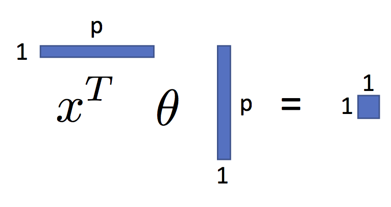
As we will see, shortly, this is a very expressive parametric model.
In previous lectures we derived the Least Squares parameter values for this model. Let's derive them once more.
Matrix Notation
Before we proceed we need to define some new notation to describe the entire dataset. We introduce the design (covariate) matrix $X$ and the response matrix (vector) $Y$ which encode the data:
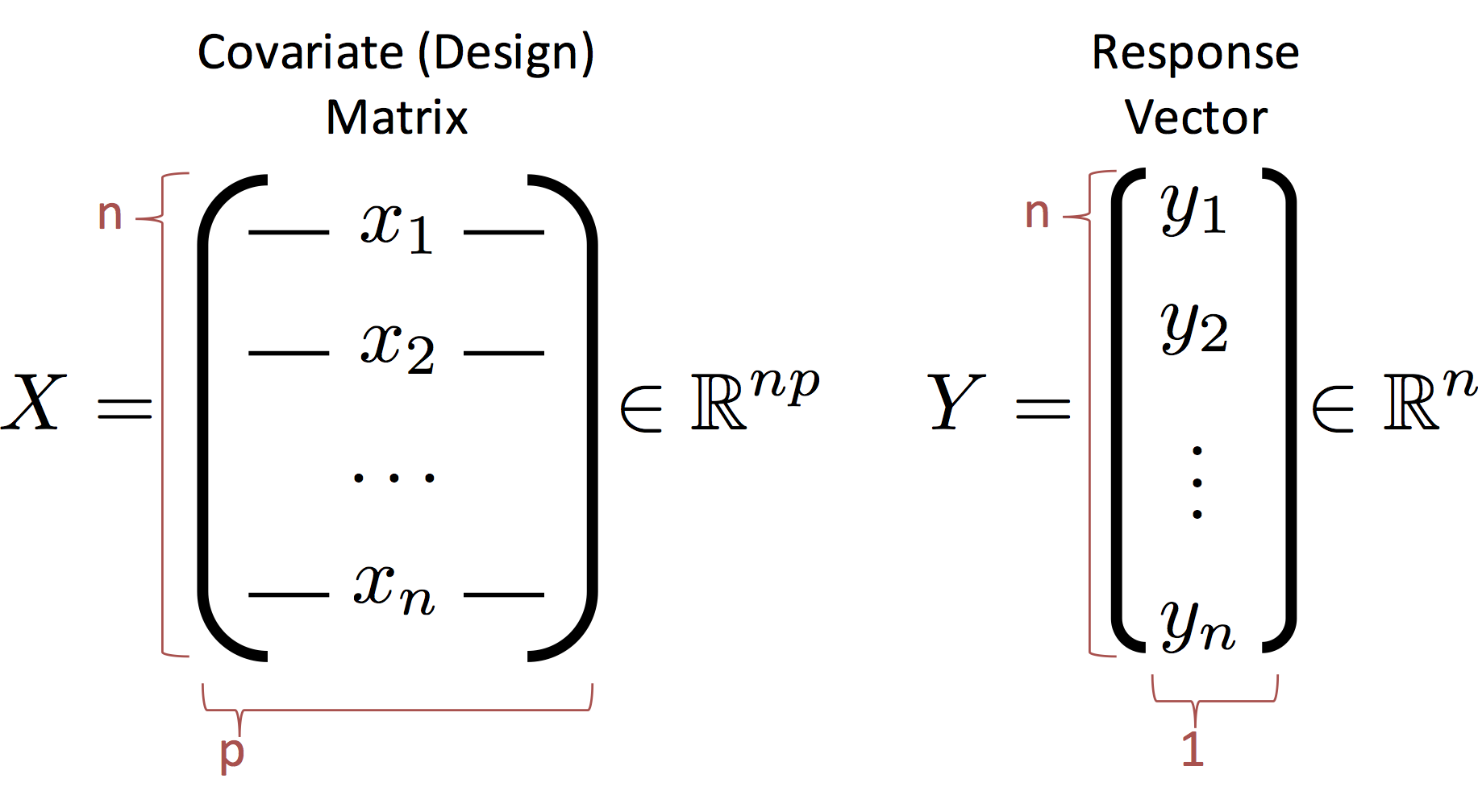
Notes:
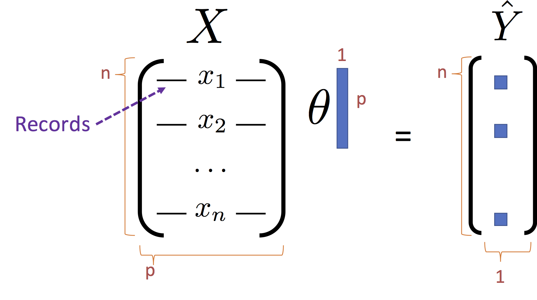
- The rows of $X$ correspond to records (e.g., users in our database)
- The columns of $X$ correspond to features (e.g., the age, income, height).
- CS and Stats Terminology Issue (p=d): In statistics we use $p$ to denote the number of columns in $X$ which corresponds to the number of parameters in the corresponding linear model. In computer science we use $d$ instead of $p$ to refer to the number of columns. The $d$ is in reference to the dimensionality of each record. You can see the differences in focus on the model and the data. If you get confused just flip the paper (or your computer) upside down and it will make more sense.
The Least Squares Loss Objective
We can write the loss using the matrix notation:
\begin{align} \large L_D(\theta) & \large = \frac{1}{n}\sum_{i=1}^n \left(Y_i - f_\theta(X_i)\right)^2 \\ & \large = \frac{1}{n}\sum_{i=1}^n \left(Y_i - X_i^T \theta \right)^2 \\ & \large = \frac{1}{n}\left(Y - X \theta \right)^T \left(Y - X \theta \right) \end{align}Note that the last line $X_i \theta$ is the dot product of the
Expanding the Loss
We can further simply the last expression by expanding the product:
\begin{align} \large L_D(\theta) & \large = \frac{1}{n}\left(Y - X \theta \right)^T \left(Y - X \theta \right) \\ & \large = \frac{1}{n}\left(Y^T - \left(X \theta\right)^T \right) \left(Y - X \theta \right) \\ & \large = \frac{1}{n}\left(Y^T \left(Y - X \theta \right) - \left(X \theta\right)^T \left(Y - X \theta \right) \right) \\ & \large = \frac{1}{n}\left( Y^T Y - Y^T X \theta - \left(X \theta \right)^T Y + \left(X \theta \right)^T X \theta \right) \\ & \large = \frac{1}{n} \left( Y^T Y - 2 Y^T X \theta + \theta^T X^T X \theta \right) \end{align}Note: Because $\left(X \theta \right)^T Y$ is a scalar it is equal to its transpose $Y^T X \theta$ and therefore $- Y^T X \theta - \left(X \theta \right)^T Y = -2 Y^T X \theta$.
Computing the Loss Minimizing $\theta$
Recall our goal is to compute:
\begin{align} \large \hat{\theta} = \arg \min_\theta L(\theta) \end{align}Which we can compute by taking the gradient of the loss and setting it equal to zero.
\begin{align} \large \nabla_\theta L(\theta) & \large = \frac{1}{n} \left( \nabla_\theta Y^T Y - \nabla_\theta 2 Y^T X \theta + \nabla_\theta \theta^T X^T X \theta \right) \end{align}To complete this expression we will need some basic gradient identities.
The first two identities we will use:
- $\large \nabla_\theta \left( A \right) = 0$ which allows us to compute $\large \nabla_\theta Y^T Y = 0$
- $\large \nabla_\theta \left( A \theta \right) = A^T$ which allows us to compute $\large \nabla_\theta 2 Y^T X \theta = \left( 2 Y^T X \right)^T = 2 X^T Y$
The remaining quadratic gradient identity:
- $\large \nabla_\theta \left( \theta^T A \theta \right) = A\theta + A^T \theta$ allows us to compute: $$ \large \nabla_\theta \theta^T X^T X \theta = X^T X \theta + (X^T X)^T \theta = 2 X^T X \theta $$
Thus we get the final gradient value:
\begin{align} \large \nabla_\theta L(\theta) & \large = \frac{1}{n} \left( \nabla_\theta Y^T Y - \nabla_\theta 2 Y^T X \theta + \nabla_\theta \theta^T X^T X \theta \right) \\ & \large = \frac{1}{n} \left( 0 - 2 X^T Y + 2 X^T X \theta \right) \end{align}Setting the gradient equal to zero we get the famous Normal Equations:
$$\large X^T X \theta = X^T Y $$$$\large \theta = \left(X^T X\right)^{-1} X^T Y $$The Normal Equation
The normal equations define the least squares optimal parameter value $\hat{\theta}$ for the linear regression model:
$$\large \hat{\theta{}} = \left(X^T X\right)^{-1} X^T Y $$and have the pictorial interpretation of the matrices:
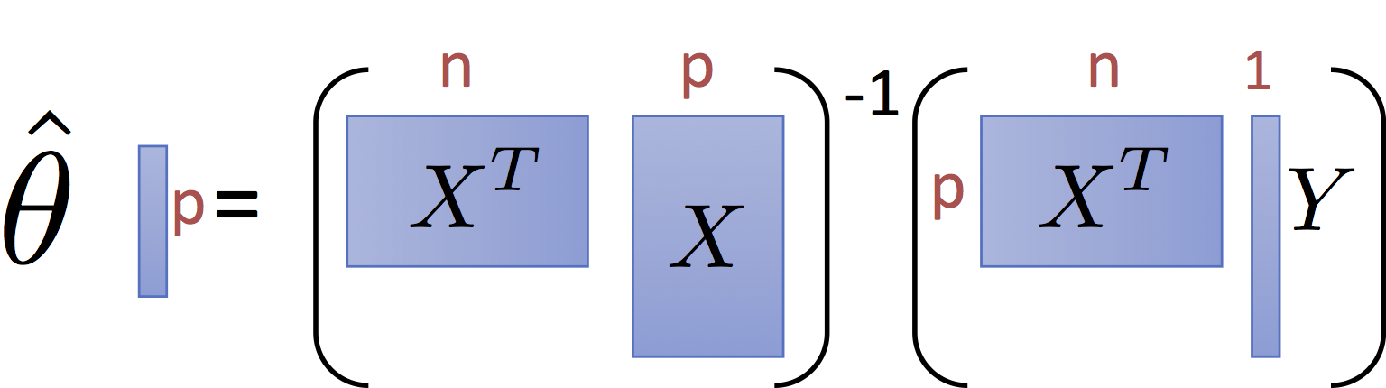
It is worth noting that for common settings where $n >> p$ (i.e., there are many records and only a few dimensions) the matrix $X^T X$ and $X^T Y$ are small relative to the data. That is they summarize the data.
Toy Data
For this exercise we are going to use synthetic data to illustrate the basic ideas of model design. Notice here that we are generating data from a linear model with Gaussian noise.
train_data = pd.read_csv("data/toy_training_data.csv")
train_data.head()
# Visualize the data ---------------------
train_points = go.Scatter(name = "Training Data",
                          x = train_data['X'], y = train_data['Y'],
                          mode = 'markers')
# layout = go.Layout(autosize=False, width=800, height=600)
py.iplot(go.Figure(data=[train_points]),
         filename="L19_b_p1")
Solving the Normal Equations
There are several ways to compute the normal equations.
Extracting the Data as Matrices
# Note that we select a list of columns to return a matrix (n,p)
X = train_data[['X']].values
print("X shape:", X.shape)

Y = train_data['Y'].values
print("Y shape:", Y.shape)
Adding the ones column
phiX = np.hstack([X, np.ones(X.shape)])
phiX[1:5,:]
Solving for $\hat{\theta{}}$
There are multiple ways to solve for $\hat{\theta{}}$. Following the solution to the normal equations:
$$\large \hat{\theta{}} = \left(X^T X\right)^{-1} X^T Y $$we get:
theta_hat = np.linalg.inv(phiX.T @ phiX) @ phiX.T @ Y
theta_hat
However computing inverting and multiplying (i.e., solving) can be accomplished with a special routine more efficiently:
$$\large A^{-1}b = \texttt{solve}(A, b) $$theta_hat = np.linalg.solve(phiX.T @ phiX, phiX.T @ Y)
theta_hat
Using a Package to estimate the linear model
In practice, it is generally better to use specialized software packages for linear regression. In Python, scikit-learn is the standard package for regression.
![]()
Here we will take a very brief tour of how to use scikit-learn for regression. Over the next few weeks we will use scikit-learn for a range of different task.
You can use the the scikit-learn linear_model package to compute the normal equations. This package supports a wide range of generalized linear models. For those who are interested in studying machine learning, I would encourage you to skim through the descriptions of the various models in the linear_model package. These are the foundation of most practical applications of supervised machine learning.
from sklearn import linear_model
Intercept Term Scikit-learn can automatically add the intercept term. This can be helpful since you don't need to remember to add it later when making a prediction. In the following we create a model object.
line_reg = linear_model.LinearRegression(fit_intercept=True)
We can then fit the model in one line (this solves the normal equations.
# Fit the model to the data
line_reg.fit(train_data[['X']], train_data['Y'])
np.hstack([line_reg.coef_, line_reg.intercept_])
Examining the solution
In the following we plot the solution along with it's residuals.
Making Predictions Using Linear Algebra
Making predictions at each of the training data points.
y_hat = phiX @ theta_hat
We can also use the trained model to render predictions.
y_hat = line_reg.predict(train_data[['X']])
Visualizing the fit
To visualize the fit line we will make a set of predictions at 10 evenly spaced points.
X_query = np.linspace(train_data['X'].min()-1, train_data['X'].max() +1, 1000)
phiX_query = np.hstack([X_query[:,np.newaxis], np.ones((len(X_query),1))])
y_query_pred = phiX_query @ theta_hat
We can then plot the residuals along with the line.
# Define the least squares regression line
basic_line = go.Scatter(name = r"Linear Model", x=X_query, y = y_query_pred)

# Definethe residual lines segments, a separate line for each
# training point
residual_lines = [
    go.Scatter(x=[x,x], y=[y,yhat],
               mode='lines', showlegend=False,
               line=dict(color='black', width = 0.5))
    for (x, y, yhat) in zip(train_data['X'], train_data['Y'], y_hat)
]

# Combine the plot elements
py.iplot([train_points, basic_line] + residual_lines)
Examining the Residuals
It is often helpful to examine the residuals. Ideally the residuals should be normally distributed.
residuals = train_data['Y'] - y_hat
sns.distplot(residuals)

We might also plot $\hat{Y}$ vs $Y$. Ideally, the data should be along the diagonal.
# Plot.ly plotting code
py.iplot(go.Figure(
    data = [go.Scatter(x=train_data['Y'], y=y_hat, mode='markers', name="Points"),
            go.Scatter(x=[-10, 50], y = [-10, 50], name="Diagonal")],
    layout = dict(title=r"Y_hat vs Y Plot", xaxis=dict(title="Y"),
                  yaxis=dict(title=r"$\hat{Y}$"))
))
The sum of the residuals should be?
np.sum(residuals)
Plotting against dimensions in X
When plotted against any one dimension we don't want to see any patterns:
# Plot.ly plotting code
py.iplot(go.Figure(
    data = [go.Scatter(x=train_data['X'], y=residuals, mode='markers')],
    layout = dict(title="Residual Plot", xaxis=dict(title="X"),
                  yaxis=dict(title="Residual"))
))
Applying Kernel regression we can look for patterns in the data:
from sklearn.kernel_ridge import KernelRidge

# Use Kernelized Ridge Regression with Radial Basis Functions to
# compute a smoothed estimator.  Later in this notebook we will
# actually implement part of this  ...
clf = KernelRidge(kernel='rbf', alpha=2)
clf.fit(train_data[['X']], residuals)
residual_smoothed = clf.predict(np.reshape(X_query, (len(X_query),1)))
# Plot the residuals with with a kernel smoothing curve
py.iplot(go.Figure(
    data = [go.Scatter(name = "Residuals",
                       x=train_data['X'], y=residuals,
                       mode='markers'),
            go.Scatter(name = "Smoothed Approximation",
                       x=X_query, y=residual_smoothed,
                       line=dict(dash="dash"))],
    layout = dict(title="Residual Plot", xaxis=dict(title="X"),
                  yaxis=dict(title="Residual"))
))
Solving Normal Equations when $n$ is big
To solve the normal equations we need to compute the following:
$$\large A = X^T X = \sum_{i=1}^n X_i^T X_i = \sum_{i=1}^n \left(\begin{matrix} X_{i,1}^2 & X_{i,1} X_{i,2} & \ldots & X_{i,1} X_{i,p} \\ X_{i,2} X_{i,1} & X_{i,2}^2 & \ldots & X_{i,2} X_{i,p} \\ \vdots & \vdots & \vdots & \vdots \\ X_{i,p} X_{i,1} & X_{i,p} X_{i,2} & \ldots & X_{i,p}^2 \end{matrix}\right) \in \mathbb{R}^{p \times p} $$$$\large b = X^T Y = \sum_{i=1}^n X_i^T Y_i = \sum_{i=1}^n \left(\begin{matrix} X_{i,1} Y_i \\ X_{i,2} Y_i \\ \vdots \\ X_{i,p} Y_i \end{matrix}\right) \in \mathbb{R}^{p} $$Note that both $A$ and $b$ are order $p$ and they can be written as a sum over $n$. In the homework you will have the opportunity to compute these in map reduce. Once $A$ and $b$ are computed we can then use np.linalg.solve to complete the calculation locally on our computer since we are assuming $p$ is relatively small. If $p$ is not small than we will need to modify the model and the solver. More on this in future lectures.
Distributed Calculation
Here we simulate distributed computing library by using the built-in sum and map operations in Python3
XtX = sum(map(lambda x: np.outer(x, x),  phiX))
XtY = sum(map(lambda xy: xy[0] * xy[1],  zip(phiX, Y)))
Local Calculation
The values of $X^T X$ and $X^T Y$ are small:
print("XtX:\n", XtX)
print("XtY:\n", XtY)
np.linalg.solve(XtX, XtY)